A relational database would be unusable without indexes: WHERE employee_id = 42 on a billion rows needs a B-tree to jump straight to the row instead of scanning every one. Vector search has the same problem in a harder form. We are not looking for an exact value but for the nearest vectors in hundreds of dimensions, and classical index structures do not help with that. This chapter covers the indexes that do.
Flat index: exact, and slow at scale
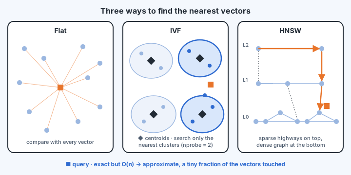
The simplest "index" is no index at all. Store every vector in a list, and for each query compute the similarity with every stored vector, then keep the top k. This is called a flat (or brute-force) index.
- It is exact: it always finds the true nearest neighbours, so recall is 100%.
- Its cost grows linearly with the corpus. A thousand vectors take microseconds, but a hundred million vectors of 1,536 dimensions means about 150 billion multiply-adds per query.
For a few thousand or even a few hundred thousand chunks, flat search is perfectly good, and it is the gold standard against which approximate methods are measured. Beyond that, we need to stop looking at most of the data.
Approximate nearest neighbours (ANN)
The idea behind every scalable vector index is to accept a small chance of missing a true neighbour in return for examining only a small fraction of the vectors. These are approximate nearest-neighbour (ANN) methods. Their quality is measured by recall@k: of the true k nearest neighbours (as a flat search would find them), what fraction did the index return? A good ANN index reaches 95–99% recall while scanning well under 1% of the data.
IVF: search only the nearest clusters
The inverted file index (IVF) works like a library organised into sections.
- Build: run k-means over the stored vectors to form, say, 1,000 clusters. Each cluster has a centroid, its average vector. Every vector is filed under its nearest centroid, in an inverted list per cluster.
- Query: compare the query with the 1,000 centroids only, pick the nearest one, and search exhaustively inside that cluster.
Instead of a billion comparisons we make about a thousand (centroids) plus about a million (one cluster's members).
The weakness is at the boundaries. If the query sits near the edge between two clusters, its true neighbours may have been filed in the neighbouring cluster, and searching only one cluster misses them entirely. The standard fix is a parameter usually called nprobe: search the nearest several clusters instead of one. With nprobe = 1 the search is fastest and recall is lowest, and raising nprobe increases recall in exchange for more work. IVF is very memory-friendly, and it combines well with compression (below).
HNSW: walk a layered graph
Hierarchical Navigable Small World (HNSW) graphs are the most widely used ANN index in vector databases today. They are fast, have high recall and handle incremental inserts well.
The structure is a multi-layer graph:
- Every vector is a node, linked to a handful of its near neighbours.
- The bottom layer contains all nodes, densely connected.
- Each higher layer contains a random, progressively smaller subset, so the top layers are sparse and provide long-range "highways".
A search works like reading maps at increasing zoom: country map, then state, then city, then street.
- Enter at the top layer, then greedily hop to whichever neighbour is closest to the query until no neighbour is closer.
- Drop down one layer from that spot and repeat, now with finer, denser links.
- In the bottom layer, run a slightly wider search and return the best k.
Because the sparse upper layers cover large distances in a few hops, a search touches only a tiny fraction of the nodes. "Small world" refers to the property, familiar from social networks, that any two nodes are connected by a short chain of links.
The three settings that matter
| Parameter | When it acts | Higher value means |
|---|---|---|
| M: links per node | Build | Better connectivity and higher recall, but more memory and slower inserts |
| efConstruction: candidate list size while building | Build | Better-quality graph and higher recall, but slower index build |
| efSearch: candidate list size while searching | Query | Higher recall, but slower queries |
Typical starting values are M ≈ 16–32 and efConstruction ≈ 100–200. efSearch is the one you tune in production, because you can change it per query without rebuilding: raise it until recall@k on your evaluation set levels off, then stop. Each further increase only adds latency.
HNSW's main cost is memory. The graph and the full vectors normally live in RAM, which becomes expensive at hundreds of millions of vectors.
Hybrids and compression
Large deployments combine these ideas.
- Cluster first, then graph. Partition the vectors into clusters (as IVF does) and build a smaller graph, or a disk-friendly structure, within each cluster, so that only the clusters relevant to a query are loaded and walked. Some vendors ship this as a named index type (for example, Weaviate's HFresh). The goal is graph-quality recall with far less memory, and cheaper updates.
- Quantization. Store compressed vectors, for example product quantization (PQ), which replaces each segment of a vector with a short code, or simple scalar quantization from 32-bit floats to 8-bit integers. Memory drops by 4–30×, at some cost in precision. It is common to search compressed vectors, then re-score the top few hundred candidates with full-precision vectors.
Choosing an index
| Index | Recall | Speed | Memory | Best for |
|---|---|---|---|---|
| Flat | Exact | Slow at scale | Vectors only | Under ~100k vectors; ground truth for evaluation |
| IVF (+PQ) | Good, tunable via nprobe | Fast | Low | Very large corpora on a memory budget |
| HNSW | Very high, tunable via efSearch | Very fast | High | The default for most RAG systems |
| Cluster + graph | High | Fast | Moderate | Billions of vectors, frequent updates |
In practice, managed vector databases choose sensible defaults (usually HNSW) and expose only a few settings. Knowing what those settings do is what lets you diagnose the classic production complaint: "the right chunk is in the index, but search doesn't return it."
Move the query near a cluster border and raise nprobe until recall recovers.