Activation Functions: From Sigmoid to GELU

The activation function $g$ decides how a neuron's weighted sum becomes its output. The choice strongly affects whether gradients can flow through a deep network.

Trouble with sigmoid and tanh

• Saturation. For large positive or negative inputs both curves flatten out and their slope approaches zero. A saturated neuron passes almost no gradient back. The sigmoid's slope is at most 0.25 even at its steepest, so each layer shrinks the gradient by at least a factor of four (the thin-network numbers in the backpropagation module showed it).
• Not zero-centred (sigmoid). All outputs are positive, so the next layer's inputs are all positive, which makes the weight updates move in awkward all-same-sign directions. Tanh fixes this: its outputs run from $-1$ to $1$ around zero. But tanh still saturates.
• Cost. Both need an exponential, slower than a simple comparison.

ReLU

The rectified linear unit is

Its advantages explain why it took over from sigmoid and tanh in many deep networks:

• No saturation for positive inputs. The slope is exactly 1, so gradients pass through unchanged.
• Very cheap to compute.
• Sparse activity. Many neurons output exactly zero.

Its weakness is the dead neuron problem. If a neuron's input is negative for every training example, its output and its gradient are both zero, so its weights stop changing and it can stay dead for good. A large learning rate that kicks the bias far negative can cause this.

Fixes for dead neurons

• Leaky ReLU gives negative inputs a small slope instead of zero: $g(a) = a$ for $a > 0$ and $g(a) = 0.01\,a$ otherwise. A little gradient always flows.
• Parametric ReLU (PReLU) makes that slope a parameter and learns it.
• ELU (exponential linear unit) uses $g(a) = a$ for $a > 0$ and $g(a) = e^{a} - 1$ for $a \le 0$. It is smooth and approaches a constant ($-1$) for very negative inputs, which pushes the average output towards zero.

Smooth modern activations

• GELU (Gaussian error linear unit): $g(a) = a\,\Phi(a)$, where $\Phi$ is the cumulative distribution function of a standard normal. It weights the input by the probability that a standard normal variable is below it: a smooth curve that is nearly zero for negative $a$ and close to $a$ for positive $a$. It is common in Transformer models.
• SiLU (also called Swish): $g(a) = a\,\sigma(a)$, the input times its sigmoid. It looks very similar to GELU.

Both are smooth, unlike ReLU's sharp corner, and dip slightly below zero for small negative inputs before returning towards zero.

The numbers

import numpy as np
from math import erf, exp, sqrt, tanh

sigmoid = lambda a: 1 / (1 + exp(-a))
acts = {
    "sigmoid": sigmoid,
    "tanh": tanh,
    "ReLU": lambda a: max(0.0, a),
    "leaky ReLU (0.01)": lambda a: a if a > 0 else 0.01 * a,
    "ELU": lambda a: a if a > 0 else exp(a) - 1,
    "GELU": lambda a: a * 0.5 * (1 + erf(a / sqrt(2))),
    "SiLU": lambda a: a * sigmoid(a),
}
points = (-4, -2, -1, 0, 1, 2)
print(f"{'a':>18s}", "".join(f"{p:8d}" for p in points))
for name, f in acts.items():
    print(f"{name:>18s}", "".join(f"{f(p):8.3f}" for p in points))
slope = lambda f, a: (f(a + 1e-6) - f(a - 1e-6)) / 2e-6
print("slope at a = -4:", {name: round(slope(f, -4), 4) for name, f in acts.items()})
print("slope at a =  2:", {name: round(slope(f, 2), 4) for name, f in acts.items()})

Output:

a       -4      -2      -1       0       1       2
           sigmoid    0.018   0.119   0.269   0.500   0.731   0.881
              tanh   -0.999  -0.964  -0.762   0.000   0.762   0.964
              ReLU    0.000   0.000   0.000   0.000   1.000   2.000
 leaky ReLU (0.01)   -0.040  -0.020  -0.010   0.000   1.000   2.000
               ELU   -0.982  -0.865  -0.632   0.000   1.000   2.000
              GELU   -0.000  -0.046  -0.159   0.000   0.841   1.954
              SiLU   -0.072  -0.238  -0.269   0.000   0.731   1.762
slope at a = -4: {'sigmoid': 0.0177, 'tanh': 0.0013, 'ReLU': 0.0, 'leaky ReLU (0.01)': 0.01, 'ELU': 0.0183, 'GELU': -0.0005, 'SiLU': -0.0527}
slope at a =  2: {'sigmoid': 0.105, 'tanh': 0.0707, 'ReLU': 1.0, 'leaky ReLU (0.01)': 1.0, 'ELU': 1.0, 'GELU': 1.0852, 'SiLU': 1.0908}

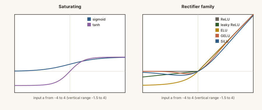
Reading the slopes at $a = 2$: sigmoid and tanh have shrunk the gradient to 0.105 and 0.071, while the rectifier family passes it through at about 1. At $a = -4$, sigmoid and tanh are nearly flat (0.018 and 0.0013), ReLU is exactly zero (a dead region), and leaky ReLU keeps a small but non-zero slope (0.01).

Choosing

• ReLU is a common default for convolutional and feedforward networks. Try leaky ReLU or ELU if dead neurons are a problem.
• GELU and SiLU are popular in large modern models, especially Transformers.
• Sigmoid is still right at the output of a binary classifier (a probability), and tanh and sigmoid appear inside gated units. But they are rarely a good choice for the hidden layers of a deep network.
• Pair the activation with a matching initialization (He for ReLU-type units).