Backpropagation Intuition: The Chain Rule on a Thin Network

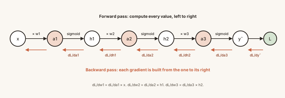
Before the general formulas, look at the smallest possible deep network. It has one neuron in every layer, so every weight is a single number and there are no matrices to confuse us.

The thin network

with squared-error loss $L = \tfrac12(\hat y - y)^2$.

We want $\partial L / \partial w_1$, the effect of the very first weight on the loss.

The chain rule, link by link

A change in $w_1$ changes $a_1$, which changes $h_1$, then $a_2$, $h_2$, $a_3$, $\hat y$ and finally $L$. The chain rule multiplies the derivative of each link:

Every factor is easy: the derivative of a sigmoid is $\sigma(1 - \sigma)$, the derivative of a product $w\,h$ with respect to $h$ is $w$, and with respect to $w$ it is $h$.

Real numbers

Take $x = 1$, $y = 1$ and weights $w_1 = 0.5$, $w_2 = -0.3$, $w_3 = 0.8$.

Forward pass: $h_1 = 0.6225$, $h_2 = 0.4535$, $\hat y = 0.5897$, loss $= 0.0842$.

The factors:

The gradients: multiplying the factors gives

To check the derivation, we nudge each weight by a tiny amount, recompute the loss and divide by the nudge. The numerical estimates are $-0.04501$, $-0.01225$ and $0.001388$, which agree with the chain-rule values.

Observation 1: work backwards and reuse

Look at how the three gradients share pieces. The first part of the product for $w_1$, namely $(\hat y - y)\,\hat y(1-\hat y)\,w_3\,h_2(1-h_2)\,w_2\,h_1(1-h_1)$, contains the first part of the product for $w_2$ as a prefix.

So instead of multiplying the whole chain again for every weight, we go backwards and keep a running product:

1. Start with $\dfrac{\partial L}{\partial \hat y}$.
2. Multiply by $\hat y (1 - \hat y)$ to get $\dfrac{\partial L}{\partial a_3}$. Now $\dfrac{\partial L}{\partial w_3} = \dfrac{\partial L}{\partial a_3}\,h_2$.
3. Multiply by $w_3$ to get $\dfrac{\partial L}{\partial h_2}$, then by $h_2(1-h_2)$ to get $\dfrac{\partial L}{\partial a_2}$. Now $\dfrac{\partial L}{\partial w_2} = \dfrac{\partial L}{\partial a_2}\,h_1$.
4. Multiply by $w_2$, then by $h_1(1-h_1)$, to get $\dfrac{\partial L}{\partial a_1}$. Now $\dfrac{\partial L}{\partial w_1} = \dfrac{\partial L}{\partial a_1}\,x$.

Each layer's gradient is built from the next layer's, using a couple of multiplications. The total work is proportional to the number of layers. That is backpropagation: the error signal flows backwards and each weight reads off its own gradient on the way.

Observation 2: gradients shrink going backwards

Look at the three results: $0.045$, $0.012$, $0.0014$. The earlier the weight, the smaller its gradient, shrinking by a factor of about 4 to 9 at each step here.

The reason is in the factors. Every step back multiplies by a weight and by a sigmoid derivative $\sigma(1-\sigma)$, which is never more than $0.25$. Multiply enough numbers smaller than 1 and the product collapses toward zero. The early layers then learn very slowly.

This is the vanishing gradient problem, which you met in the history course when we asked why deep networks stayed hard to train. Now you can see it happen in numbers, and the later remedies (other activations, better initialisation) will make sense.