Why is the test error U-shaped? The answer is an identity that splits the error into parts with clear meanings.
Two imaginary experiments
Suppose we could repeat the whole training process many times, each time with a fresh training set drawn from the same source, and see what prediction the model makes at a fixed input . Each run gives a slightly different prediction , because each training set has different noise.
Two things can be said about this collection of predictions:
- Bias. Where is their average, compared with the truth? Bias is the gap between the average prediction and the true function . A large bias means the model is systematically wrong, even on average. This happens when the model is too simple for the pattern.
- Variance. How much do the predictions spread around their own average? A large variance means the prediction depends strongly on which training set we happened to get. This happens when the model is so flexible that it follows the noise.
The decomposition
For squared error, the expected error at a new point splits exactly:
where and is the noise variance. The third term is the irreducible error: no model can predict random noise.
Measuring them
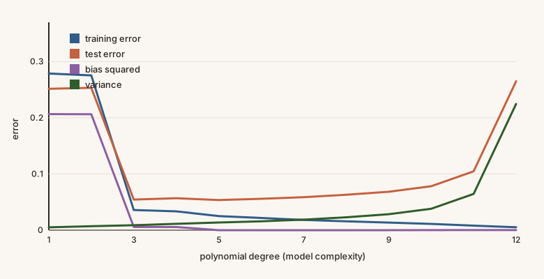
We can measure all three in our polynomial experiment, because we know the true function. For each degree, fit 1000 training sets, record the predictions on a grid of test points, and compute the bias and the variance of those predictions. We also measure the actual test error directly, to check that the parts add up.
import numpy as np
from numpy.polynomial import legendre

def true_f(x):
    return np.sin(2 * np.pi * x)

def features(x, degree):
    return legendre.legvander(2 * x - 1, degree)

def fit(x, y, degree, lam=0.0):
    A = features(x, degree)
    return np.linalg.solve(A.T @ A + (lam + 1e-9) * np.eye(degree + 1), A.T @ y)

x_train = np.linspace(0, 1, 15)
x_test = np.linspace(0.005, 0.995, 200)
noise = 0.2
rng = np.random.default_rng(1)

for degree in (1, 3, 5, 9, 12):
    preds, measured = [], []
    for _ in range(1000):
        y = true_f(x_train) + rng.normal(0, noise, 15)
        w = fit(x_train, y, degree)
        p = features(x_test, degree) @ w
        preds.append(p)
        measured.append(np.mean((p - (true_f(x_test) + rng.normal(0, noise, 200))) ** 2))
    preds = np.array(preds)
    bias_sq = np.mean((preds.mean(axis=0) - true_f(x_test)) ** 2)
    variance = np.mean(preds.var(axis=0))
    print(f"degree {degree:2d}: bias^2 {bias_sq:.4f}  variance {variance:.4f}  noise {noise**2:.4f}  sum {bias_sq + variance + noise**2:.4f}  measured test error {np.mean(measured):.4f}")
Output:
degree  1: bias^2 0.2054  variance 0.0048  noise 0.0400  sum 0.2502  measured test error 0.2499
degree  3: bias^2 0.0056  variance 0.0089  noise 0.0400  sum 0.0545  measured test error 0.0543
degree  5: bias^2 0.0000  variance 0.0135  noise 0.0400  sum 0.0535  measured test error 0.0535
degree  9: bias^2 0.0000  variance 0.0283  noise 0.0400  sum 0.0683  measured test error 0.0681
degree 12: bias^2 0.0002  variance 0.2175  noise 0.0400  sum 0.2577  measured test error 0.2569
The last two columns agree, so the decomposition works. Reading the table:
- Degree 1: nearly all the error is bias squared (0.205). The straight line cannot follow a sine wave however much data it sees, and it hardly changes between training sets (variance 0.005).
- Degrees 3 to 5: bias has almost vanished and variance is still small. This is the sweet spot.
- Degree 12: bias is essentially zero, yet the variance has exploded to 0.22. On average the model is right, but any single fit is wildly off.
The trade-off
Making a model more flexible reduces bias and increases variance. Making it simpler does the opposite. The best model balances the two, and the total is the U.
You can diagnose which side you are on:
| Symptom | Diagnosis | Things to try |
|---|---|---|
| Training error high, test error high and close to it | high bias (underfitting) | a bigger or more flexible model, better features, train longer |
| Training error low, test error much higher | high variance (overfitting) | more data, a simpler model, regularization (the rest of this module) |
More training data reduces variance without increasing bias, which is why it is the most reliable fix for overfitting when it is available. When more data is not available, regularization is the next tool.
See bias, variance and test error for every degree on one chart.