We now have a family of methods. This lesson puts them side by side, gives you code to try them, and says what you can and cannot conclude from such comparisons.
The update rules at a glance
Notation: is the gradient at the current point and all operations on vectors are element by element.
| Method | Keeps | Update | Idea |
|---|---|---|---|
| Gradient descent | nothing | step downhill | |
| Momentum | velocity | , then | build speed, damp zigzag |
| Nesterov (NAG) | velocity | same, with taken at | look ahead, brake early |
| AdaGrad | per-parameter rate, shrinking | ||
| RMSProp | = decaying average of | per-parameter rate, no shrinking | |
| AdaDelta | averages of and of | no learning rate | |
| Adam | decaying averages and | momentum plus RMSProp, bias-corrected | |
| AdaMax | and a decaying max | Adam with the max norm |
A test bed
Here is the complete code for two test problems and all eight optimisers, in one place. The problems are the ones we have used throughout: the narrow valley and the sigmoid toy problem.
import numpy as np

sigmoid = lambda z: 1 / (1 + np.exp(-z))

# ---- two test problems -------------------------------------------------
def valley_loss(t):            # narrow valley: 10 times steeper in w than in b
    return 0.5 * (10 * t[0] ** 2 + t[1] ** 2)

def valley_grad(t):
    return np.array([10 * t[0], t[1]])

X, Y = np.array([0.5, 2.5]), np.array([0.2, 0.9])      # the sigmoid toy problem

def toy_loss(t):
    return 0.5 * np.sum((sigmoid(t[0] * X + t[1]) - Y) ** 2)

def toy_grad(t):
    p = sigmoid(t[0] * X + t[1])
    c = (p - Y) * p * (1 - p)
    return np.array([np.sum(c * X), np.sum(c)])

# ---- optimisers: each returns a step(theta, grad_fn) function ------------
def make(name, eta=0.1, gamma=0.9, beta1=0.9, beta2=0.999, rho=0.95):
    s = dict(v=0.0, G=0.0, E=0.0, Ed=0.0, m=0.0, u=0.0, t=0)

    def step(theta, grad):
        g = grad(theta - gamma * s["v"]) if name == "nag" else grad(theta)
        s["t"] += 1
        if name == "gd":
            return theta - eta * g
        if name in ("momentum", "nag"):
            s["v"] = gamma * s["v"] + eta * g
            return theta - s["v"]
        if name == "adagrad":
            s["G"] = s["G"] + g ** 2
            return theta - eta * g / (np.sqrt(s["G"]) + 1e-8)
        if name == "rmsprop":
            s["E"] = 0.9 * s["E"] + 0.1 * g ** 2
            return theta - eta * g / (np.sqrt(s["E"]) + 1e-8)
        if name == "adadelta":                       # no learning rate
            s["E"] = rho * s["E"] + (1 - rho) * g ** 2
            d = -np.sqrt(s["Ed"] + 1e-6) / np.sqrt(s["E"] + 1e-6) * g
            s["Ed"] = rho * s["Ed"] + (1 - rho) * d ** 2
            return theta + d
        if name == "adam":
            s["m"] = beta1 * s["m"] + (1 - beta1) * g
            s["E"] = beta2 * s["E"] + (1 - beta2) * g ** 2
            m_hat = s["m"] / (1 - beta1 ** s["t"])
            v_hat = s["E"] / (1 - beta2 ** s["t"])
            return theta - eta * m_hat / (np.sqrt(v_hat) + 1e-8)
        if name == "adamax":
            s["m"] = beta1 * s["m"] + (1 - beta1) * g
            s["u"] = np.maximum(beta2 * s["u"], np.abs(g))
            return theta - eta / (1 - beta1 ** s["t"]) * s["m"] / (s["u"] + 1e-8)
    return step

def steps_to_settle(loss, grad, theta0, step, threshold, max_steps=3000):
    """First step after which the loss stays below the threshold, or None."""
    theta, losses = np.array(theta0, float), []
    for _ in range(max_steps + 1):
        losses.append(loss(theta))
        theta = step(theta, grad)
    losses = np.array(losses)
    if not np.isfinite(losses).all():
        return None
    above = np.where(losses >= threshold)[0]
    if len(above) == 0:
        return 0
    return int(above[-1] + 1) if above[-1] + 1 <= max_steps else None
Note the measure: the number of steps after which the loss stays below a threshold. "First time it dips below" would flatter methods that jitter.
Now run both problems:
valley_runs = [("gd", 0.18), ("gd", 0.05), ("momentum", 0.05), ("nag", 0.05), ("adagrad", 0.5),
               ("rmsprop", 0.05), ("adadelta", None), ("adam", 0.1), ("adamax", 0.1)]
print("Narrow valley, start (1, 1): steps until loss stays below 1e-4")
for name, eta in valley_runs:
    step = make(name, eta if eta else 0.1)
    print(f"  {name:9s} rate {eta}:", steps_to_settle(valley_loss, valley_grad, [1, 1], step, 1e-4))

toy_runs = [("gd", 1.0), ("momentum", 1.0), ("nag", 1.0), ("adagrad", 1.0),
            ("rmsprop", 0.1), ("adadelta", None), ("adam", 0.3), ("adamax", 0.3)]
print("Sigmoid toy problem, start (-2, -2): steps until loss stays below 1e-3")
for name, eta in toy_runs:
    step = make(name, eta if eta else 0.1)
    print(f"  {name:9s} rate {eta}:", steps_to_settle(toy_loss, toy_grad, [-2, -2], step, 1e-3))
Output (None means it did not settle within 3000 steps):
Narrow valley, start (1, 1): steps until loss stays below 1e-4
  gd        rate 0.18: 25
  gd        rate 0.05: 84
  momentum  rate 0.05: 102
  nag       rate 0.05: 49
  adagrad   rate 0.5: 10
  rmsprop   rate 0.05: None
  adadelta  rate None: None
  adam      rate 0.1: 94
  adamax    rate 0.1: 79
Sigmoid toy problem, start (-2, -2): steps until loss stays below 1e-3
  gd        rate 1.0: 183
  momentum  rate 1.0: 148
  nag       rate 1.0: 83
  adagrad   rate 1.0: 21
  rmsprop   rate 0.1: 102
  adadelta  rate None: 348
  adam      rate 0.3: 81
  adamax    rate 0.3: 51
What the results do and do not say
Read the two tables with care.
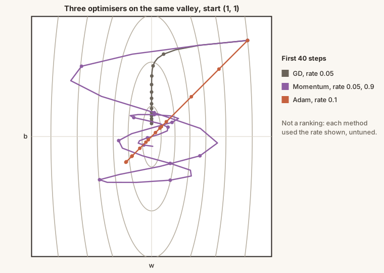
- These are tiny, smooth, convex problems, and each method used a rate that was picked by hand without careful tuning. The numbers show the mechanisms at work. They are not a ranking for real networks.
- Plain gradient descent with a well-chosen rate is hard to beat on the narrow valley (25 steps at ). On the toy problem it is slow because the start is flat and the best rate is large.
- Momentum and NAG help most when plain gradient descent is crawling; on the valley, momentum alone was slower than plain descent at the same rate. NAG settled faster than momentum on both problems.
- AdaGrad is fastest here, but partly by luck: the valley's axes line up with the parameters, and the toy problem is small and stops quickly. Its ever-shrinking rate is a weakness for long runs.
- RMSProp and AdaDelta did not settle on the valley with a constant rate. RMSProp jitters at a scale set by , and AdaDelta starts very slowly.
- Adam and AdaMax settled on both problems, at modest speed.
Sensitivity to the learning rate
The real difference shows up when we change the rate. Steps to settle on the sigmoid toy problem (none: did not settle in 3000 steps, or diverged):
| Rate | Plain GD | Momentum | RMSProp | Adam |
|---|---|---|---|---|
| 0.03 | none | 620 | 129 | 234 |
| 0.1 | 1815 | 177 | 102* | 74 |
| 0.3 | 606 | 124 | 2995* | 81 |
| 1 | 183 | 148 | none | 846 |
| 3 | 62 | none | none | none |
| 10 | 15 | none | none | none |
*RMSProp keeps jittering close to the threshold, so these two numbers are fragile: a different numerical library (or the simulator) can give a noticeably different step, for example about 160 instead of 102 at rate 0.1. Read them as "roughly a hundred steps, or barely at all".
And on the narrow valley:
| Rate | Plain GD | Momentum | RMSProp | Adam |
|---|---|---|---|---|
| 0.01 | 424 | 100 | none | 236 |
| 0.05 | 84 | 102 | none | 100 |
| 0.1 | 41 | 103 | none | 94 |
| 0.19 | 52 | 103 | none | 96 |
| 0.21 | none | 109 | none | 99 |
| 0.5 | none | none | none | 101 |
Two lessons:
- The best rate depends on the method and on the problem. Plain gradient descent needs large rates on the toy problem (its gradients are tiny) and small ones on the valley (its gradients are large). Adam's rate is a distance per step, so its sweet spot (here around 0.1 to 0.3) is more similar across the two problems.
- The adaptive methods are tolerant in a different way. They are safe over a wide band of rates, but each has an upper limit. At a rate larger than the whole problem they never settle. Plain gradient descent on the valley fails at 0.21, and on the toy problem it happily takes a rate of 10.
Practical advice
Hedged, because every problem differs:
- Adam with its default values and a rate around is a very common starting point for deep networks, because it needs little tuning.
- Mini-batch gradient descent with momentum and a good schedule is also widely used. Many practitioners find it matches Adam, or does better, on some tasks, but it needs more care with the rate.
- Tune the learning rate first. It matters more than the choice between most optimisers.
- Add a schedule. Warm-up, then decay or cosine annealing, is a common combination for large models.
- Watch the loss curve. Loss exploding means the rate is too high. A flat curve means it is too low or you are on a plateau.
- Keep it simple until you have a reason not to. Change one thing at a time so you can tell what helped.
Run all eight optimisers together on any of five loss surfaces.