From Step to Sigmoid

So far we have worked almost entirely with Boolean functions, where inputs and outputs are 0 or 1. Real problems rarely look like that, so we now move to functions $y = f(x)$ where both $x$ and $y$ are real numbers.

Real inputs, real outputs

Suppose an oil company must decide whether to build a drilling station at a location in the ocean. The decision depends on many measurements: salinity, density, pressure, temperature, marine diversity. Each is a real number, so the input is a vector $x \in \mathbb{R}^n$. The quantity we want to predict, the amount of oil that could be extracted, is also a real number, $y \in \mathbb{R}$.

Other examples have the same shape:

• Interest rate for a loan. Inputs are salary, family size, past loans, past defaults. The output is a rate, say between 5% and 20%.
• Images. A 100 by 100 grey image is just 10,000 pixel values, a very long input vector, and the output might be a label or score.

For Boolean functions we asked whether a network could represent the function exactly. For real functions we relax that: can a network represent it approximately, so that its output $\hat y$ is close to the true $y$ for the examples we have? That is the quest for the rest of this module.

The step function is too harsh

Recall how a perceptron decides: it fires when the weighted sum of its inputs passes a threshold. Take a movie decision based on a single input, the critics' rating on a 0 to 1 scale, with threshold 0.5.

• A film rated 0.49 gives output 0: dislike.
• A film rated 0.51 gives output 1: like.

A difference of 0.02 flips the decision completely. Nobody decides that way. We would expect 0.49 to be nearly as good as 0.51.

This has nothing to do with movies or with the threshold we picked. It is a property of the function itself, a step function: flat at 0, then a sudden jump to 1.

The sigmoid neuron

We replace the step with a smooth S-shaped curve. A very common choice is the logistic function:

Here $z$ is the same weighted sum as before. From now on we write the bias as $b$ (this was $w_0$, which equals $-\theta$, in the perceptron). A neuron that applies $\sigma$ to its weighted sum is a sigmoid neuron.

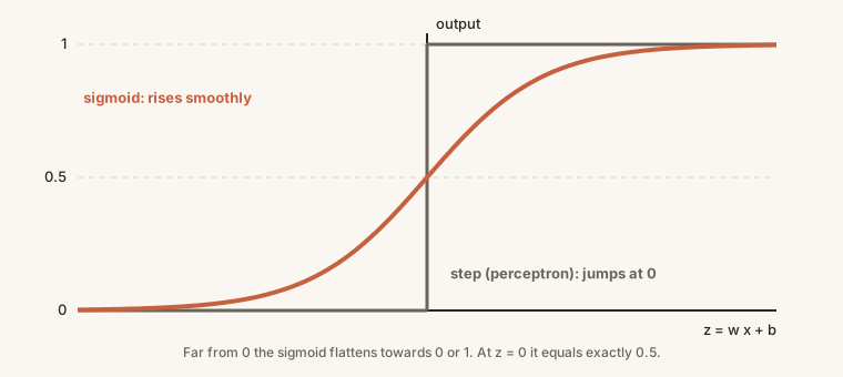
Check its behaviour by plugging in values:

• As $z \to +\infty$, $e^{-z} \to 0$, so $\sigma(z) \to 1$.
• As $z \to -\infty$, $e^{-z} \to \infty$, so $\sigma(z) \to 0$.
• At $z = 0$, $\sigma(0) = 1/(1+1) = 0.5$.

In between it rises smoothly. For example $\sigma(2) \approx 0.88$ and $\sigma(-2) \approx 0.12$. At the extremes it saturates, barely changing however large $|z|$ becomes.

With one input, $z = wx + b$, the curve is centred where $z = 0$, that is at $x = -b/w$. A larger $|w|$ makes it steeper, and as $w$ grows it approaches the step function. Changing $b$ slides it left or right.

What we gain

A graded output. The output is any number between 0 and 1, not just 0 or 1.

A probability reading. Because the output lies between 0 and 1, we can read it as a probability. An output of 0.49 means roughly a 49% chance of liking the film, and 0.51 means 51%. That is exactly the gentle behaviour the step lacked. A domain expert can then choose how to act on the probability, for example investing only above 70%.

A smooth, differentiable curve. The step is not differentiable at its jump, and everywhere else its slope is zero. The sigmoid has a slope at every point. This matters enormously: for much of this course, calculus is the main tool, and the learning algorithm ahead needs derivatives.

The logistic function is one member of the sigmoid family of S-shaped functions. Another, $\tanh$, appears later in the course.