The update rule needs two numbers at each step, and . We now derive them for our sigmoid neuron and then run the algorithm.
The loss for one example
The model is . For a single training example the loss is
Derivative with respect to
Use the chain rule. The derivative of a square is twice the thing times the derivative of the thing, and the cancels the 2:
The true value is a constant, so it contributes nothing to the derivative. What remains is the derivative of the sigmoid. Write . The sigmoid is , so
This is a neat property: the derivative of the sigmoid is expressed using the sigmoid's own output. With and the chain rule factor :
Putting it together:
Derivative with respect to
The same steps apply, except , so the factor disappears:
Many examples
With examples the loss is a sum, and the derivative of a sum is the sum of the derivatives:
Notice how much is shared: the two formulas differ only by the final .
In code
We train on the toy data from before, the points and , starting from with learning rate :
import numpy as np

X = np.array([0.5, 2.5])
Y = np.array([0.2, 0.9])

def f(x, w, b):
    return 1 / (1 + np.exp(-(w * x + b)))

def loss(w, b):
    return 0.5 * np.sum((f(X, w, b) - Y) ** 2)

def gradients(w, b):
    pred = f(X, w, b)
    common = (pred - Y) * pred * (1 - pred)   # shared by both derivatives
    return np.sum(common * X), np.sum(common)

w, b, eta = -2.0, -2.0, 1.0
for epoch in range(1, 1001):
    dw, db = gradients(w, b)
    w -= eta * dw
    b -= eta * db
    if epoch in (1, 10, 100, 500, 1000):
        print(epoch, round(w, 3), round(b, 3), round(loss(w, b), 5))
Output:
1 -1.995 -1.992 0.41573
10 -1.942 -1.92 0.41484
100 1.003 -1.051 0.01774
500 1.785 -2.272 0.0
1000 1.792 -2.282 0.0
Reading the run
- The loss only goes down. Unlike guesswork, no step takes us uphill.
- The start is slow. From the gradient is tiny, about , because both sigmoids are saturated there. The loss barely moves in the first ten epochs (0.4157 to 0.4148). Then the path reaches steeper ground and the loss drops fast. By epoch 100 it is 0.018.
- It ends where we wanted. The final , is almost exactly the parameter pair we reached by hand earlier, , and the loss is essentially 0.
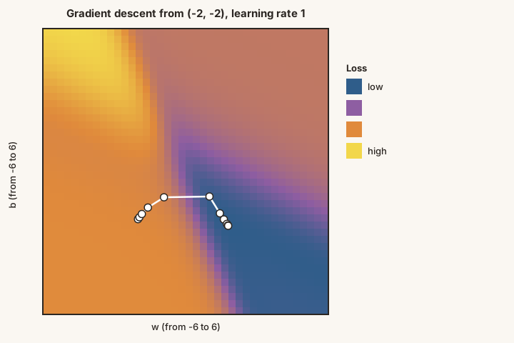
Run gradient descent on a loss surface and watch the point roll towards the minimum.
Completing the cycle
The story now mirrors the perceptron's:
| Perceptron | Sigmoid neuron | |
|---|---|---|
| Model | step on a weighted sum | sigmoid on a weighted sum |
| Error | misclassified points | squared-error loss |
| Learning algorithm | perceptron learning algorithm | gradient descent |
| Ran it and watched it converge | yes | yes |
Next, as we did for the perceptron, we ask what this kind of neuron can represent.