Guesswork and the Error Surface

Fit a sigmoid to two points by trial and error, measure each guess with the loss, and see that you were walking on an error surface without a map.

Before building a proper algorithm, try the obvious thing: guess, measure, adjust. It teaches exactly what a good algorithm must improve on.

A toy problem

Keep the model as small as possible: one input and one sigmoid neuron,

\hat f(x) = \frac{1}{1 + e^{-(wx + b)}}

and only two training examples:

$x$	$y$
0.5	0.2
2.5	0.9

We want $w$ and $b$ so that the S-shaped curve passes close to both points. In other words, $\hat f(0.5) \approx 0.2$ and $\hat f(2.5) \approx 0.9$ .

The loss is the squared error from the last lesson, $L(w, b) = \tfrac12 \sum_i (\hat f(x_i) - y_i)^2$ .

Start with a guess

Take $w = 3$ , $b = -1$ . The predictions are $\hat f(0.5) = \sigma(0.5) \approx 0.62$ and $\hat f(2.5) = \sigma(6.5) \approx 0.998$ . Both are off: the curve passes above both points. To say how wrong, plug into the loss:

L(3, -1) = \tfrac12\left[(0.62 - 0.2)^2 + (0.998 - 0.9)^2\right] \approx 0.094

A perfect fit would give 0. Now any guess can be scored.

Keep guessing, guided by the loss

Guess $(w, b)$	Predictions at 0.5 and 2.5	Loss	Verdict
(3, −1)	0.62, 0.998	0.094	start
(0.5, 0)	0.56, 0.78	0.073	better
(−0.1, 0)	0.49, 0.44	0.148	worse: made $w$ negative
(0.94, −0.94)	0.39, 0.80	0.022	much better
(1.78, −2.27)	0.20, 0.90	below 0.0001	essentially perfect

The reasoning behind these steps went like this. The first change reduced the loss. The third increased it, so making $w$ negative was a bad idea. After that, raising $w$ and lowering $b$ helped, so keep going that way. The loss was giving feedback, and we were using it.

The error surface

Because we can compute $L$ for any $(w, b)$ , we can plot it over the plane of all parameter values. The height at each point is the loss. This is the error surface (or loss surface) we met earlier, now for a sigmoid neuron.

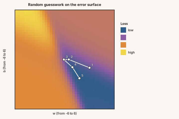
Colour map of the loss for every pair of w and b, with the path of the guesses drawn on top and numbered — The loss for every (w, b). Dark blue is low. The numbered points are the five guesses from the table, in order.

Plotted this way, what we did is clear. Guess 1 sat in a high-loss region. We jumped around, at one point climbing to a worse spot (guess 3), then luckily landed in the dark valley. We were navigating the surface blindly.

Try it yourself

Error surfaces in 3D →

Rotate a loss surface and find the valley yourself.

Why guesswork does not scale

We only got there because we could see a two-point, two-parameter example and because we knew roughly where to go. In general:

We cannot try every value. Each parameter can be any real number. The plot above shows only $-6$ to $6$ , and there might be a lower valley just outside it.
Computing the loss everywhere is too expensive. The cost grows quickly with the number of examples and, far worse, with the number of parameters. Real networks have millions.
Random jumps waste effort and can go uphill. We want every move to reduce the loss.

What we need is a principled way to decide, at the current point, which direction to move so the loss goes down, and by how much. That is what the next three lessons develop.

EasyLoss

Compute the loss for w = 0, b = 0 on this data.

EasyError surface

In the guess table, the guess (-0.1, 0) had a higher loss than the one before it. What does that tell you?

MediumError surface