Plain gradient descent works, but it can be slow or unstable. To understand why, and how the methods in this module fix it, we need a way to look at loss surfaces on a flat page. That tool is the contour plot.
From a surface to a map
A loss surface is a landscape: the height above each point is the loss. A contour plot is the same landscape seen from directly above, the way a hiking map shows a hill. Each closed curve, a contour line or level curve, joins all the points with the same loss value.
Reading one is like reading a hiking map:
- Rings close together mean the ground changes quickly: the surface is steep.
- Rings far apart mean the ground is nearly flat.
- The smallest ring is at the bottom of the bowl, the minimum.
- Moving along a contour, the loss does not change. Moving across contours, it does.
The gradient is perpendicular to the contour
Along a contour line the loss stays constant, so the slope in that direction is zero. The gradient, which points in the direction of steepest increase, therefore has no component along the contour. It must be perpendicular to it, pointing across the contour towards higher loss.
A gradient descent step is the opposite direction: straight across the contour lines, downhill.
A narrow valley
We will use one test surface again and again in this module:
It has its minimum at . The loss changes ten times faster along than along . The contours are ellipses stretched along the direction, a long narrow valley with steep walls.
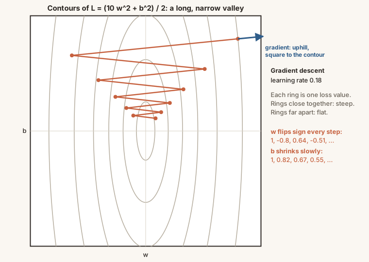
The gradient is , so gradient descent updates each coordinate separately:
Take from the start :
| Step | ||
|---|---|---|
| 0 | 1 | 1 |
| 1 | −0.8 | 0.82 |
| 2 | 0.64 | 0.67 |
| 3 | −0.51 | 0.55 |
| 4 | 0.41 | 0.45 |
| 5 | −0.33 | 0.37 |
The steep coordinate flips sign at every step (it is multiplied by ), which is the zigzag across the valley. The gentle coordinate shrinks by a factor of 0.82 and makes steady but slow progress.
Why you cannot just raise the rate
The steep direction sets a speed limit. shrinks only if , so we need . At the factor is , the zigzag grows, and gradient descent diverges. With a smaller rate such as the path is smooth, but is multiplied by 0.95 each step and crawls.
For a bowl like this there is a best choice, , which is where we started. Even then each step shrinks both coordinates by only a factor of , where is the ratio of the steepest to the gentlest curvature. On this surface that still finishes quickly: the loss stays below after 25 steps (), against 84 steps with .
But the ratio can be huge for real networks. With , the best factor is , and shrinking an error by a factor of takes thousands of steps. Steep in one direction and flat in another is the core difficulty that the methods in this module attack, in different ways.
Flat regions too
Contours also explain the slow start we saw for the sigmoid neuron. Near the starting point the rings are far apart: the surface is nearly flat, the gradient is tiny (), and gradient descent barely moves. A method that builds up speed on flat ground would escape sooner. That is the idea of momentum, in the next lesson.
Read the contour map, click to choose a start, and watch gradient descent cross the valley.