Until now the learning rate has been one fixed number. Yet the ideal step size changes during training. Early on we want large steps to cover ground quickly. Near the end we want small steps so the parameters can settle instead of bouncing around the minimum. A schedule changes as training goes on.
Decay schedules
The simplest idea is to start with a rate and shrink it. Three common forms, where is the step number:
| Schedule | Formula | Behaviour |
|---|---|---|
| Step decay | constant for steps, then multiplied by (for example halved every 20 steps) | |
| Exponential decay | smooth, fast shrink | |
| Inverse-time decay | smooth, slower shrink |
With , halving every 20 steps, for the exponential and for inverse-time, the rates at a few steps are:
| Step | Step decay | Exponential | Inverse-time |
|---|---|---|---|
| 0 | 0.1 | 0.1 | 0.1 |
| 20 | 0.05 | 0.055 | 0.05 |
| 50 | 0.025 | 0.022 | 0.029 |
| 100 | 0.003 | 0.005 | 0.017 |
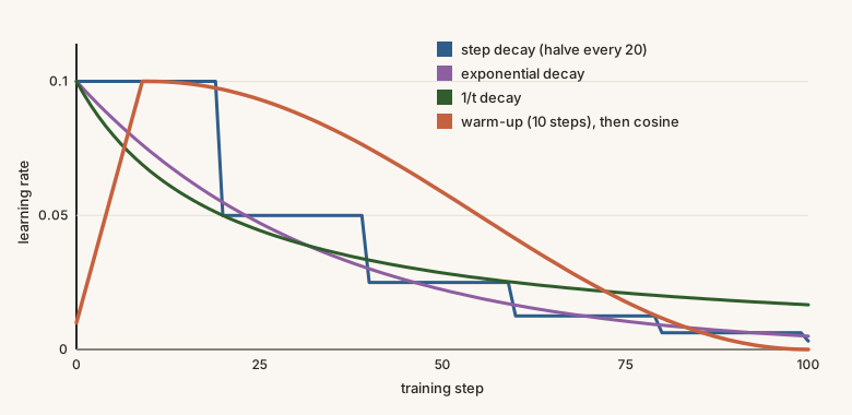
The decay speed is a hyperparameter like any other. Too fast and training stalls before it has finished learning. Too slow and the noise near the end is not reduced.
Line search: choosing the rate each step
Instead of a fixed plan, we can search for a good step size at every update. Take the gradient direction and try a large step. If it does not reduce the loss enough, shrink it and try again. A standard test, the backtracking rule, accepts when
for a small constant such as : the loss must drop by a fixed fraction of what the slope predicts. Start with and halve until the test passes.
On the narrow valley, starting from , this rule picks different rates at different steps:
| Iteration | Rate chosen | Loss after the step |
|---|---|---|
| 1 | 0.125 | 0.695 |
| 2 | 0.125 | 0.313 |
| 3 | 0.25 | 0.209 |
| 4 | 0.25 | 0.192 |
| 5 | 0.125 | 0.077 |
| 6 | 0.25 | 0.054 |
| 7 | 0.25 | 0.054 |
| 8 | 0.125 | 0.019 |
The loss started at 5.5 and falls at every step without us choosing a rate by hand. The price is extra loss evaluations in every trial. For a large network each trial costs a forward pass over the data, and with mini-batches the loss is itself noisy, so line search is rarely used for training deep networks. Fixed schedules are cheaper.
Warm-up
Sometimes the start is the dangerous part. At the very beginning the weights are random, gradient estimates can be wild, and methods that keep running averages (like those in the coming lessons) have had little data to average. A large rate right away can throw training off.
Warm-up starts with a tiny rate and raises it linearly to the target over the first steps:
Cosine annealing
After warm-up, we can lower the rate smoothly along a half cosine wave, from down to over steps:
It falls slowly at first, fastest in the middle, and slowly again at the end, which lets the parameters settle gently. Some schemes restart the cosine cycle several times.
With , , and , the rate at steps 0, 4, 9, 10, 32, 55 and 99 is
It ramps up, peaks at step 10, and then declines to zero by the end. A warm-up followed by cosine decay is a very common recipe for training large networks.
In code
import math

def step_decay(k, eta0=0.1, drop=0.5, every=20):
    return eta0 * drop ** (k // every)

def warmup_cosine(t, eta_max=0.1, eta_min=0.0, warmup=10, total=100):
    if t < warmup:
        return eta_max * (t + 1) / warmup
    progress = (t - warmup) / (total - warmup)
    return eta_min + 0.5 * (eta_max - eta_min) * (1 + math.cos(math.pi * progress))

print([round(warmup_cosine(t), 3) for t in (0, 4, 9, 10, 32, 55, 99)])
Inside a training loop, just set eta = warmup_cosine(step) before each update.
Pick a learning rate schedule and see how it calms RMSProp near the minimum.