So far every gradient was computed from the whole training set: the loss is a sum over examples and so is its gradient. With 1,000 examples that is fine. With millions, each update would be very expensive. The fix is to estimate the gradient from a small sample.
Three flavours
Let be the number of examples used for each parameter update.
| Name | Updates per pass over the data | |
|---|---|---|
| Batch gradient descent | all | 1 |
| Stochastic gradient descent (SGD) | 1 | |
| Mini-batch gradient descent | in between, for example 32 |
One full pass through the training data is an epoch. All three methods see every example once per epoch. They differ in how often they update.
Why a sample is good enough
The full gradient is the average of the per-example gradients. If you pick examples at random, the average over a small sample is a noisy but unbiased estimate of it: on average it points in the right direction. A few dozen examples already give a rough idea of which way is downhill, at a fraction of the cost.
The price is noise. Each step follows a slightly different, slightly wrong direction, so the path jitters.
An experiment
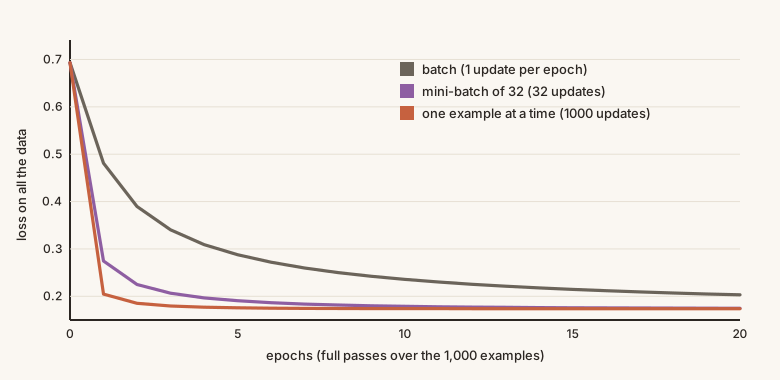
We generate 1,000 points from two overlapping blobs and fit a logistic regression (a single sigmoid neuron) with cross-entropy loss. Each method uses its own learning rate, chosen sensibly: 0.5 for batch, 0.1 for mini-batches of 32, 0.01 for single examples. The loss is measured on all the data after each epoch:
| Method | Updates per epoch | Loss after 1 epoch | after 2 | after 5 | after 20 |
|---|---|---|---|---|---|
| Batch | 1 | 0.481 | 0.3897 | 0.2878 | 0.2031 |
| Mini-batch (32) | 32 | 0.2745 | 0.225 | 0.1907 | 0.1747 |
| One at a time | 1000 | 0.2047 | 0.1853 | 0.1757 | 0.1738 |
The accuracy of all three stays between 92% and 93% throughout. The difference is speed per epoch: after a single epoch, batch descent has made one step and is at 0.48, while mini-batch and single-example updates have already made good progress.
The code
import numpy as np

sigmoid = lambda z: 1 / (1 + np.exp(-z))

data_rng = np.random.default_rng(0)
n = 1000
X = np.vstack([data_rng.normal([-1, -1], 1.0, (n // 2, 2)),     # two overlapping blobs
               data_rng.normal([1, 1], 1.0, (n // 2, 2))])
y = np.r_[np.zeros(n // 2), np.ones(n // 2)]

def full_loss(w, b):                                            # cross-entropy on ALL the data
    p = sigmoid(X @ w + b)
    return -np.mean(y * np.log(p + 1e-12) + (1 - y) * np.log(1 - p + 1e-12))

def train(batch_size, eta, epochs):
    shuffle_rng = np.random.default_rng(1)
    w, b = np.zeros(2), 0.0
    losses = []
    for epoch in range(epochs):
        order = shuffle_rng.permutation(n)                      # shuffle every epoch
        for start in range(0, n, batch_size):
            j = order[start:start + batch_size]                 # one mini-batch
            p = sigmoid(X[j] @ w + b)
            g = p - y[j]                                        # gradient of cross-entropy
            w -= eta * (X[j].T @ g) / len(j)
            b -= eta * g.mean()
        losses.append(full_loss(w, b))
    return losses

for name, size, eta in [("batch", 1000, 0.5), ("mini-batch", 32, 0.1), ("one at a time", 1, 0.01)]:
    L = train(size, eta, epochs=20)
    print(name, [round(float(L[k - 1]), 4) for k in (1, 2, 5, 20)])
Output:
batch [0.481, 0.3897, 0.2878, 0.2031]
mini-batch [0.2745, 0.225, 0.1907, 0.1747]
one at a time [0.2047, 0.1853, 0.1757, 0.1738]
Setting batch_size = n gives batch descent and batch_size = 1 gives SGD. Two habits are worth copying: shuffle every epoch, so batches are not always the same, and average the gradient over the batch, so the learning rate means the same thing for any batch size.
Trade-offs
- Noise. Small batches give noisy gradients. The loss does not settle exactly and keeps wobbling around the minimum. Reducing the learning rate over time (next lesson) calms this.
- Hardware. Computers do matrix operations on many examples far more efficiently than one example at a time, so mini-batches usually use the hardware better than pure SGD.
- Cost per update. A small batch is cheap, so many more updates fit into the same time.
In practice, mini-batches of 32 to 256 examples are the standard choice, and people often say "SGD" for mini-batch gradient descent. The momentum and adaptive methods in this module apply to mini-batch gradients exactly as they do to full ones.
Train the same network with batch sizes of all, 32, 8 and 1, and compare the curves.