Taylor Series: Approximating a Curve Locally

We want to change the parameters $\theta = (w, b)$ by a small amount and have the loss go down. To know what a move will do without trying it, we need a way to predict the loss near where we stand. The Taylor series is that tool.

The idea in one variable

Take a loss $L(w)$ with a single parameter. Suppose we know its value at a point $w_0$, and we want its value at a nearby point $w$. The linear approximation says

Here $L'(w_0)$ is the derivative, the slope of the curve at $w_0$. In words: the new value is the old value plus the slope times the distance moved.

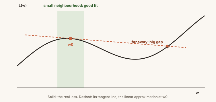
This is just the equation of a straight line. If $y = mx + c$, then $y_1 - y_0 = m(x_1 - x_0)$, so $y_1 = y_0 + m(x_1 - x_0)$, where $m$ is the slope. We have replaced the curve by its tangent line at $w_0$ and read off the line's height at $w$.

It only works nearby

Look at the figure. In the small shaded neighbourhood, the line and the curve are almost indistinguishable. Move far from $w_0$, and the line drifts away from the curve: the approximation is poor. Two things control the size of the error:

• How far you move. The smaller the step $|w - w_0|$, the better the approximation.
• How fast the slope changes. Where the curve is almost flat, a straight line fits well over a wide window. Where the curve is steep or bending quickly, the same window gives a much larger error.

Adding more terms

We can do better than a line by keeping more terms of the series:

Stopping after the first-derivative term gives a linear (first-order) approximation. Stopping after the second-derivative term gives a quadratic one, a parabola that hugs the curve more closely and stays accurate over a wider window. Adding more terms improves the fit further. If you keep every term (for well-behaved functions), you get the function back exactly.

As a check, approximating $\sin x$ near a point: a line fits only a narrow stretch, a parabola covers a bit more, and with degree 7 or 8 the polynomial follows the sine curve over a wide range.

Two variables

Our loss depends on two parameters, $L(w, b)$. The same idea works:

• the linear approximation is a flat plane touching the surface at the current point,
• the quadratic approximation is a curved, bowl-like surface.

Again, in a small neighbourhood the plane is a good match for the surface. Move far away and it is not. The same rules hold in any number of dimensions, even though we cannot draw them.

Why this matters

We will keep only the linear terms and use a small step. Then we can say, for any proposed move, how much the loss will change, using only the slope at the current point. That is enough to choose a direction that reduces the loss. The next lesson does exactly that, and it explains why the step size is called a learning rate and kept small.