The Backpropagation Algorithm

All the pieces are in place. Backpropagation is two sweeps through the network and then an ordinary gradient descent update.

The algorithm

Forward pass. Starting from $h_0 = x$, for $k = 1, \dots, L-1$ compute and store

then $a_L = b_L + W_L h_{L-1}$ and $\hat y = O(a_L)$.

Backward pass.

1. At the output, $\delta_L = \hat y - e_\ell$ (softmax with cross-entropy).
2. For $k = L, L-1, \dots, 1$:
   1. $\nabla_{W_k} L = \delta_k\,h_{k-1}^{T}$ and $\nabla_{b_k} L = \delta_k$
   2. if $k > 1$: $\delta_{k-1} = \bigl(W_k^{T}\delta_k\bigr) \odot g'(a_{k-1})$

Update. For every parameter, $W_k \leftarrow W_k - \eta\,\nabla_{W_k}L$ and $b_k \leftarrow b_k - \eta\,\nabla_{b_k}L$.

Repeat over the training examples, many times.

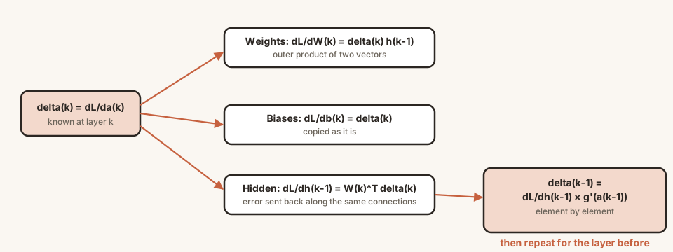
In code

The forward function is the one from the notation lesson. The backward pass follows the pseudocode line by line:

def backward(label, as_, hs, y_hat, Ws):
    """Gradients of the cross-entropy loss for one example."""
    L = len(Ws)
    dWs, dbs = [None] * L, [None] * L

    da = y_hat.copy()
    da[label] -= 1                      # delta_L = y_hat - one_hot(label)

    for k in range(L - 1, -1, -1):
        dWs[k] = np.outer(da, hs[k])    # delta_k times h_(k-1) transposed
        dbs[k] = da                     # bias gradient is delta_k
        if k > 0:
            dh = Ws[k].T @ da                   # send the error back
            da = dh * hs[k] * (1 - hs[k])       # times sigmoid slope
    return dWs, dbs

(Indices here are zero-based: Ws[k] maps hs[k] to as_[k].)

Trust, but check: the gradient check

Backpropagation is easy to get subtly wrong. A reliable test is to compare its gradients with slow numerical ones. For each parameter $\theta_i$, nudge it up and down by a tiny $\epsilon$ and use

On the worked 2-2-2 network, the largest difference between backpropagation and the numerical gradient, over all 12 parameters, is about $10^{-10}$. They agree.

One update with $\eta = 0.5$ reduces the loss on that example from $0.4716$ to $0.2559$.

Training a network on XOR

In the perceptron module we saw that one perceptron cannot learn XOR. Here is the payoff: a network with a hidden layer, trained by backpropagation, can.

def train(sizes, seed, eta, epochs):
    rng = np.random.default_rng(seed)
    Ws = [rng.normal(0, 1, (sizes[i + 1], sizes[i])) for i in range(len(sizes) - 1)]
    bs = [np.zeros(sizes[i + 1]) for i in range(len(sizes) - 1)]

    X = np.array([[0, 0], [0, 1], [1, 0], [1, 1]], dtype=float)
    Y = [0, 1, 1, 0]                                    # XOR labels

    for epoch in range(1, epochs + 1):
        dW = [np.zeros_like(W) for W in Ws]
        db = [np.zeros_like(b) for b in bs]
        total_loss = 0
        for x, label in zip(X, Y):
            as_, hs, y_hat = forward(x, Ws, bs)
            total_loss += -np.log(y_hat[label])
            gW, gb = backward(label, as_, hs, y_hat, Ws)
            for k in range(len(Ws)):
                dW[k] += gW[k]
                db[k] += gb[k]
        for k in range(len(Ws)):                        # one update per epoch
            Ws[k] -= eta * dW[k]
            bs[k] -= eta * db[k]
        if epoch in (1, 100, 500, 1000, 3000):
            print(epoch, round(total_loss, 4))

    return [int(np.argmax(forward(x, Ws, bs)[2])) for x in X]

print(train(sizes=[2, 4, 2], seed=0, eta=0.5, epochs=3000))

Output:

1 3.3434
100 2.5434
500 0.0254
1000 0.0087
3000 0.0021
[0, 1, 1, 0]

The network is 2 inputs, 4 hidden sigmoid neurons and 2 softmax outputs. The loss, summed over the four examples, falls from 3.3 to 0.002, and the predictions match XOR exactly. With seeds 1, 2 and 3 we got the same predictions.

Three details worth noticing:

• Random starting weights. If all weights began equal (for example zero), every hidden neuron would compute the same thing and receive the same gradient, so they would stay identical forever. Random starts break the symmetry.
• Slow start, then a drop. The loss barely moves for a while and then falls quickly, the same plateau-then-slope pattern we saw with the single neuron.
• Full-batch updates. This code sums the gradient over all four examples and updates once per epoch. Other schemes update after each example or after small groups, and we meet them later.

Why this is efficient

The backward pass does a few matrix operations per layer, about the same order of work as the forward pass. It produces the gradient for every parameter at once. That is the reason a network with millions of parameters can be trained at all.