Underfitting, Overfitting and Test Error

Everything so far aimed at one thing: make the training loss small. But the real goal is different. We want the model to do well on new data it has never seen. This module is about the gap between the two.

Training error and true error

The training error is the loss on the examples we used to fit the model. The true error (also called the generalisation error) is the loss we would see on fresh examples drawn from the same source. We can never compute the true error exactly, but we can estimate it.

Hold some data back and never use it for fitting. After training, measure the loss on it. For regression with squared error:

over $M$ test examples. Because the model never saw them, this is an honest, unbiased estimate of the true error. Two rules keep it honest:

• Never train on the test set.
• Never use it to make choices, such as picking a learning rate or a model size. Every choice made by looking at the test score leaks information into the model. Use a separate validation set for choices, and touch the test set once, at the very end.

An experiment: fitting a curve with polynomials

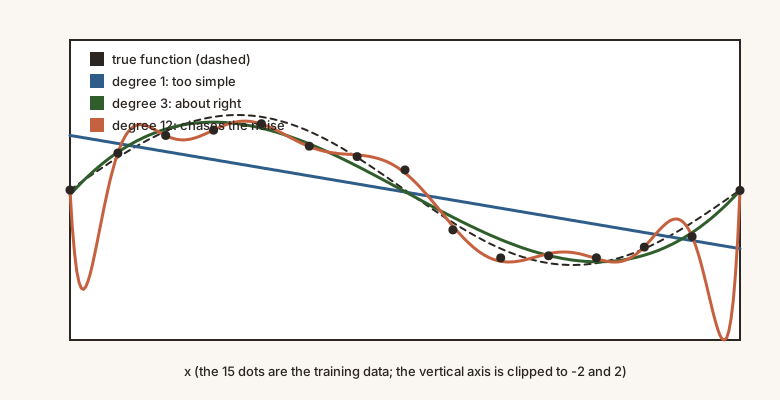
We need a setting where we can see exactly what happens. The true function is $y = \sin(2\pi x)$. We get 15 noisy measurements, with noise of standard deviation 0.2, at evenly spaced $x$ values. Then we fit polynomials of different degrees. A polynomial of degree $d$ has $d + 1$ adjustable coefficients, so higher degree means a more flexible model.

import numpy as np
from numpy.polynomial import legendre

def true_f(x):                       # the function we are trying to learn
    return np.sin(2 * np.pi * x)

def features(x, degree):             # Legendre polynomials: a well-behaved polynomial basis on [0, 1]
    return legendre.legvander(2 * x - 1, degree)

def fit(x, y, degree, lam=0.0):      # least squares (ridge when lam > 0)
    A = features(x, degree)
    return np.linalg.solve(A.T @ A + (lam + 1e-9) * np.eye(degree + 1), A.T @ y)

rng = np.random.default_rng(0)
x_train = np.linspace(0, 1, 15)      # the same 15 input positions every time
x_test = np.linspace(0.005, 0.995, 200)
noise = 0.2

for degree in (1, 3, 5, 9, 12):
    train_err, test_err = [], []
    for _ in range(1000):            # 1000 different noisy training sets
        y = true_f(x_train) + rng.normal(0, noise, 15)
        w = fit(x_train, y, degree)
        train_err.append(np.mean((features(x_train, degree) @ w - y) ** 2))
        y_new = true_f(x_test) + rng.normal(0, noise, 200)          # fresh noisy measurements
        test_err.append(np.mean((features(x_test, degree) @ w - y_new) ** 2))
    print(f"degree {degree:2d}: training error {np.mean(train_err):.4f}   test error {np.mean(test_err):.4f}")

Output, averaged over the 1000 training sets:

degree  1: training error 0.2782   test error 0.2502
degree  3: training error 0.0369   test error 0.0543
degree  5: training error 0.0237   test error 0.0537
degree  9: training error 0.0136   test error 0.0678
degree 12: training error 0.0056   test error 0.2622

The noise alone contributes $0.2^2 = 0.04$ to every test error, so 0.04 is the best any model could hope for.

Look at how the two columns behave:

• The training error only goes down as the degree rises. A more flexible model can always fit the training points at least as well.
• The test error goes down, then up. It is lowest around degrees 3 to 5 (about 0.054), and at degree 12 it has grown almost fivefold to 0.26 even though the training error is tiny.

Underfitting and overfitting

• Underfitting (degree 1). The model is too simple to capture the pattern. The error is high on both training and test data, and they are close.
• A good fit (degrees 3 to 5). The model captures the pattern but not the noise.
• Overfitting (degree 12). The model is flexible enough to memorise the noise in the training points. The training error is excellent, but the model's predictions between the points wander, so the test error is bad. There is a large gap between test and training error.

The first clue to which case you are in is to compare the two numbers. High on both: underfitting. Low training error with much higher test error: overfitting.

Why complexity matters

Model complexity, or capacity, is how rich a family of functions the model can represent: the degree of the polynomial, the number of parameters, the number of layers and neurons in a network. The same pattern holds for neural networks:

• too little capacity: the network cannot fit even the training data,
• too much capacity for the amount of data: it fits everything, noise included.

The true error is therefore a U-shaped function of complexity, with the best model in the middle. The next lesson explains why, using bias and variance. The lessons after that cover tools that let us use a flexible model and avoid overfitting.