Unsupervised Pre-training and Autoencoders

In the history of this subject, deep networks stayed hard to train until the mid-2000s. One of the ideas that broke through was to give the network a good starting point learned from data without labels.

The revival in 2006

Around 2006, Geoffrey Hinton and colleagues showed that a deep network could be trained by first pre-training it, one layer at a time, without any labels, and only then fine-tuning the whole thing with backpropagation. This unsupervised pre-training was widely credited with restarting interest in deep learning.

Why would it help? Labelled data is scarce, but unlabeled data (raw images, text, audio) is plentiful. A network can learn something about the structure of the inputs from unlabeled data alone. Weights that have already learned useful features make a far better starting point than random numbers: gradient descent starts near a region of good solutions, and the learned structure acts as a mild regularizer. (Later studies found that pre-training helped both optimization and generalisation, and that the benefit was largest when labelled data was limited.)

Autoencoders

The tool most often used is the autoencoder: a network trained to reproduce its own input.

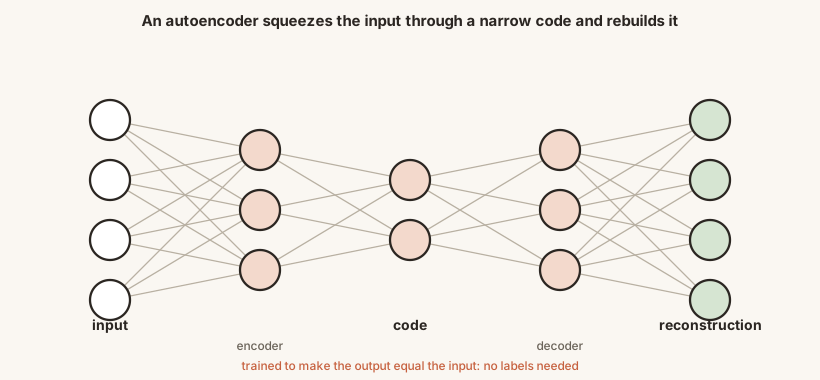
• The encoder maps the input $x$ to a code $h$ that is smaller than $x$.
• The decoder maps $h$ back to a reconstruction $\hat x$.
• The loss is the reconstruction error $\lVert \hat x - x\rVert^2$. The target is the input itself, so no labels are needed.

Because the code is narrower than the input (a bottleneck), the network cannot simply copy its input. It must discover what matters about the data and keep only that.

An example

Generate 500 points in four dimensions that really depend on only two hidden factors $z_1, z_2$: the coordinates are $z_1$, $z_2$, $z_1 + z_2$ and $z_1 - z_2$, plus a little noise. The data has four numbers per example but only two degrees of freedom. Train a linear autoencoder with code sizes 1, 2 and 4:

import numpy as np

rng = np.random.default_rng(0)
n = 500
z = rng.normal(0, 1, (n, 2))                                     # two hidden factors
X = np.column_stack([z[:, 0], z[:, 1], z[:, 0] + z[:, 1], z[:, 0] - z[:, 1]]) + rng.normal(0, 0.05, (n, 4))

def train_autoencoder(code_size, epochs=3000, eta=0.05, seed=1):
    r = np.random.default_rng(seed)
    We = r.normal(0, 0.3, (4, code_size)); Wd = r.normal(0, 0.3, (code_size, 4))
    for _ in range(epochs):
        code = X @ We                                           # encoder (linear)
        recon = code @ Wd                                       # decoder (linear)
        err = recon - X
        grad_Wd = code.T @ err / n
        grad_We = X.T @ (err @ Wd.T) / n
        Wd -= eta * grad_Wd
        We -= eta * grad_We
    return np.mean((X @ We @ Wd - X) ** 2)

print("variance of the data per coordinate:", round(float(X.var(axis=0).mean()), 4))
for size in (1, 2, 4):
    print(f"code size {size}: reconstruction error {train_autoencoder(size):.4f}")

Output:

variance of the data per coordinate: 1.4297
code size 1: reconstruction error 0.7008
code size 2: reconstruction error 0.0012
code size 4: reconstruction error 0.0010

• Code size 1: the error stays at 0.70. One number cannot describe two independent factors.
• Code size 2: the error collapses to 0.0012. The network discovered the two hidden factors and rebuilds all four coordinates from them. What is left is just the noise in the two directions it discards: the added noise has variance $0.05^2 = 0.0025$ per coordinate, and discarding two of four directions leaves about half of that.
• Code size 4: no real improvement (0.0010), because there is nothing more to capture.

The code is a compressed, learned representation of the data. That is the kind of feature one would like as a starting point for a classifier.

Layer-wise pre-training

For deep networks the recipe (in its classic form) is:

1. Train an autoencoder on the raw inputs. Keep its encoder layer.
2. Pass all the data through that encoder to get codes. Train a second autoencoder on those codes. Keep its encoder.
3. Repeat for as many layers as you want, building a stack of encoders, each trained on the output of the one before.
4. Add an output layer for the real task and fine-tune the whole stack with backpropagation on the labelled data.

Training one shallow layer at a time avoids the vanishing gradient problem of training a deep stack from random weights all at once. Hinton's original version used a related model called the restricted Boltzmann machine instead of an autoencoder, and variants such as denoising and sparse autoencoders add noise or a sparsity penalty to force better features.

Why it is used less today

Pre-training was a workaround for a problem we have since attacked directly. Better initialization (the last lesson), ReLU-type activations (the next lesson), much larger labelled datasets, faster hardware and improved optimizers mean that deep networks can often be trained well from scratch.

The idea has not gone away. Modern language models are pre-trained on huge amounts of unlabeled text and then fine-tuned for specific tasks. The details differ, but the recipe is the one from this lesson: learn general structure from plentiful unlabeled data, then specialise.