From the Top of the Stack to the Next Token

Our token's vector has travelled up the whole stack, gathering context and being refined at every block. At the top sits a $d$-dimensional vector that is the model's fully-considered summary of "what should come after this position." This last chapter turns that vector into an actual next token.

From a vector to a score per token

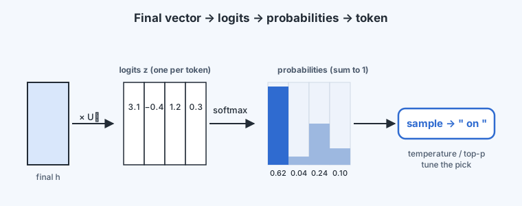
To predict the next token we need a number for every token in the vocabulary — a score saying how well each one fits. That is one matrix multiply. The final vector $h$ is multiplied by an unembedding matrix $U$ of shape $d \times V$ (one column per vocabulary token):

Each score $z_i$ is, in effect, how aligned the final vector is with token $i$'s direction. These raw scores are called logits. They are unbounded real numbers — some positive, some negative — and not yet probabilities.

From scores to probabilities: softmax

To turn the logits into a probability distribution we apply the softmax function, which exponentiates each score and normalizes:

Exponentiating makes every value positive and sharpens the gap between large and small logits; dividing by the sum makes the values add to 1. Now we have exactly the distribution from the very first chapter — a probability for every token — and this is also the quantity the training loss scores. Softmax and its cross-entropy loss are the same pair covered in the Deep Learning course's output and loss functions lesson; a language model just applies them over a vocabulary of tens of thousands.

Choosing a token

With a distribution in hand, how do we pick? The choice is a knob, not a fixed rule.

• Greedy / argmax. Take the single most probable token. Deterministic and often repetitive.
• Sampling. Draw a token at random according to the probabilities, so a token with probability 0.1 is chosen about 10% of the time. This gives variety and more natural text.

Two controls shape sampling:

Temperature $T$ rescales the logits before softmax, $z_i / T$:

• $T < 1$ sharpens the distribution — the model becomes more confident and conservative.
• $T > 1$ flattens it — more surprising, more diverse, and eventually incoherent.
• $T \to 0$ recovers greedy argmax.

Top-p (nucleus) sampling keeps only the smallest set of top tokens whose probabilities sum to $p$ (say 0.9), and samples from those — cutting off the long tail of implausible tokens while still allowing variety among the plausible ones.

The loop closes

The chosen token is appended to the input, and the entire journey runs again on the now-longer sequence to produce the token after that. Predict, append, predict — the autoregressive loop from the first chapter, now filled in end to end:

1. Tokenize the text into IDs.
2. Embed each ID into a vector (plus position, from Module 5).
3. Refine every vector up the stack of transformer blocks.
4. Unembed the final vector into logits, softmax into probabilities.
5. Sample a token, append it, and go back to step 1.

That is a complete language model. Everything remaining in the course makes this loop faster, bigger, and cheaper — but the loop itself does not change.