How Multi-Token Prediction Is Built

The last chapter said a model predicts the next $k$ tokens at each position. This one shows the machinery that does it, and the single design choice that separates the modern version from the original. As always, concepts and shapes — no code.

Start from the shared trunk

Every prediction, near or far, begins the same way: the input tokens pass up through the model's stack of transformer blocks — the shared trunk — producing a refined hidden vector at each position, exactly as in the base model. For single-token prediction, each position's hidden vector goes through one output projection (the unembedding) to give the next-token probabilities. One output step, one predicted token.

To predict $k$ tokens we need $k$ prediction steps. The naive version just bolts on $k$ output modules, each responsible for one future position: module 1 predicts the next token, module 2 the token after that, and so on, all reading from the same trunk hidden state. This is the original design — independent heads, each forecasting its own depth in parallel.

What each prediction module needs

A module predicting the token at some future depth is given two things:

• The hidden state carried into it — a summary of everything known so far.
• The input embedding of the token at that future position — available during training because the whole sentence is present.

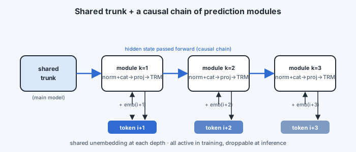
Inside the module these are combined (each normalised, then concatenated), projected back down to the model's width, passed through a small transformer layer, and finally sent through a shared unembedding to produce that depth's token probabilities. "Shared" because the same output projection serves every depth — there is no need for a separate vocabulary projection per module. The loss at each depth is the ordinary cross-entropy against that depth's true token, and the losses are summed.

The key design choice: a causal chain, not independent heads

Here is the refinement that makes the modern version better. In the original design the $k$ heads are independent: each forecasts its depth straight from the trunk, unaware of the others. That is simple, but it throws away a dependency — predicting the token three steps ahead ought to benefit from having "committed" to the token one and two steps ahead.

The modern design makes the modules sequential, linked in a causal chain. The hidden state produced by the module for depth 1 is fed as input to the module for depth 2, whose hidden state feeds depth 3, and so on. Each further-ahead prediction is conditioned on the nearer ones, so the model forecasts a coherent continuation rather than $k$ disconnected guesses. This keeping of the "complete causal chain" across depths is the chief improvement the modern version added to the original multi-token idea, and it reportedly gives better results — intuitively, because information from each prediction flows forward into the next, exactly as real text unfolds.

A detail at the edges

One small bookkeeping point: near the end of a training sequence there is not enough text left to supply $k$ future targets. A position only $2$ tokens from the end cannot be asked to predict $3$ tokens ahead. So the multi-token loss is applied only at positions that have a full horizon of real tokens after them — the last few positions simply predict fewer, or are left out of the deeper losses. It does not change the idea, but it is why the deepest prediction covers slightly fewer positions than the shallowest.

Training on, inference off

Finally, recall the practical stance from the last chapter, now visible in the architecture. The prediction modules sit on top of the shared trunk. During training they are all active, contributing their summed loss and improving the trunk's weights. At inference, if you only want the quality gains, you keep just the trunk and its first output — the ordinary next-token path — and drop the extra modules entirely. The scaffolding did its job during training; the deployed model is a normal autoregressive model that happens to have been trained with a richer objective. (Keep the modules instead, and you have a ready-made drafter for speculative decoding.)

With that, we have covered the three big levers of modern efficiency: compressing the KV cache (Module 6), scaling the FFN sparsely (Module 7), and enriching the training signal (this module). The next module turns to a lever that cuts across all of them — doing the arithmetic itself in lower precision: quantization.