The last two lessons made a model cheaper by changing how its numbers are stored. There are two other ways to get the bill down, and both are blunter: take some of the model away, or rebuild it smaller from scratch. Together with quantization these three make up the model compression family, and they are studied side by side because they are all answering the same question — how do you serve a model this capable without paying for the whole of it?
The pressure is inference, not training
A model is trained once and served endlessly, so the cost that dominates its life is inference. Four things get worse as a model grows:
- Hardware. Weights have to fit in memory. Past a certain size, serving means buying more accelerators, which puts the model out of reach for most organisations.
- Latency. A bigger model takes longer to produce each token. Users who wait seconds for a chat reply leave — and modern systems rarely make a single call. An agentic loop that generates, runs the result, reflects on the output and tries again multiplies the wait by the number of turns.
- Cost per request. If serving a user costs more than the user is worth, nothing else about the model matters. A few points of accuracy are often not worth several times the price.
- Energy. Serving at scale consumes real power and cooling, and the carbon that comes with them.
This is why every major lab ships small models alongside their flagships. The small ones typically give up a few points on benchmarks while costing a fraction as much to run — and still beat the previous generation's large model. For most products that is an easy trade, and compression is how it is made.
The techniques here are lossy: they change the model and give back a little accuracy for a lot of cost. A separate family of methods is lossless — better engineering of the same computation. Fusing attention's scale, mask, softmax and multiply into one GPU kernel, for instance, produces bit-identical results while cutting time and memory traffic sharply (you met one such method as Flash Attention). Good serving systems use both: efficient kernels because they are free, compression because kernels alone are not enough.
Three levers, three different bargains
| What it changes | Accuracy cost | Effort | Needs training data? | |
|---|---|---|---|---|
| Quantization | Bits per number | Small | Low | No |
| Pruning | Which weights exist | Small to moderate | Low to medium | Only to recover accuracy |
| Distillation | The architecture itself | Smallest, if done well | Highest | Yes |
Distillation preserves quality best and is by far the most expensive, because it means running the large model over a large dataset and then training a new one. Quantization and pruning are cheap and need little or no retraining, but each gives back a bit more quality. The right choice depends on how much speed-up you need and what you have: a target latency, a hardware generation, a dataset.
Quantization at serving time
The previous lessons looked at low precision during training. At serving time the same idea appears in two forms.
Post-training quantization (PTQ) takes a finished model and converts it, with no retraining. The architecture is untouched, so there is no design decision to make. Weights are easy: they are fixed, so their scale factors can be computed once and stored. Activations are harder, because they depend on the input — one batch may be modest, the next may contain a value far outside the range the scales assumed, and clipping it loses information. The standard fix is a calibration set: push a small sample of representative inputs through the network, record the range each activation actually takes, and set the scales from that.
In use, quantization is applied operation by operation rather than once: take the inputs and weights for a matrix multiply, quantize both, multiply in the low-bit format, then dequantize the result for whatever comes next. The conversions cost something, but low-bit tensor arithmetic is enough faster — hardware datasheets quote several times the throughput for 8-bit over 16-bit operations — that the net win is large.
Quantization-aware training (QAT) instead exposes the model to quantization while it is still learning, so the weights adapt to the coarser grid rather than being rounded onto it afterwards. The best-known example is QLoRA, which fine-tunes through a 4-bit base model; we return to it in the fine-tuning lesson, since it is as much an adaptation technique as a compression one.
When INT8 serving was first tried on growing models, quality held up to roughly a few billion parameters and then fell away sharply, while 16-bit stayed flat. The cause was outlier features: in large models a handful of activation dimensions carry values vastly larger than the rest. Scaling a vector by its maximum then crushes every ordinary value onto almost the same quantized level, and the information is gone. The remedy was to stop forcing them through the same path — detect the few outlier dimensions by threshold, keep those in 16-bit, quantize everything else to 8-bit, and add the two results. The outliers are rare enough that the cost is negligible and the quality gap closes. It is the same insight as the fine-grained scaling from the previous lesson: never let one extreme value set the scale for numbers it has nothing to do with.
Pruning: delete what is not carrying weight
Pruning removes parameters from a trained network and hopes the rest can cover for them. It comes in two kinds, and the difference between them is almost entirely about hardware.
Unstructured pruning removes individual weights wherever they are. The simplest version, magnitude pruning, sorts the weights and zeroes the smallest ones, on the reasoning that a weight near zero was contributing little. It works better than it sounds: removing a substantial fraction of weights — commonly around 40% — often costs very little accuracy, and fine-tuning after pruning recovers much of what was lost, pushing the workable fraction considerably higher.
A refinement notes that magnitude alone is the wrong measure. A weight matters only through what it multiplies, so a small weight that consistently meets a large activation may count for more than a large weight that meets near-zero inputs. Scoring weights by their interaction with observed activations prunes more accurately for the same sparsity.
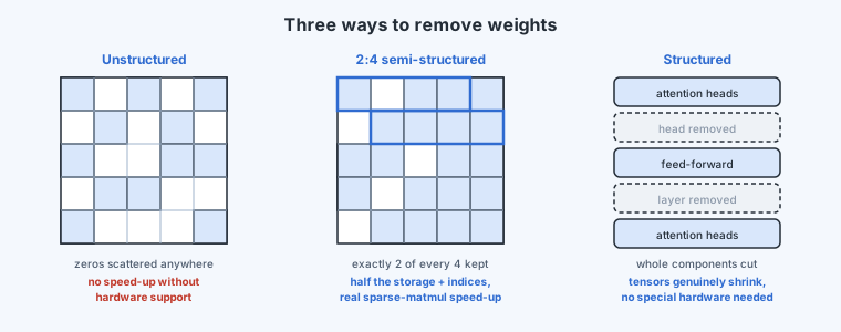
Here is the catch that shapes the whole field. A zero stored in the same format is still a number. If the hardware multiplies it like any other value, an unstructured-pruned model occupies the same memory, performs the same operations and draws the same power as before. The sparsity is real mathematically and worthless practically.
That pushes practitioners toward patterns the hardware can act on:
- Semi-structured sparsity. Recent accelerators support a 2:4 pattern — in every block of four consecutive weights, exactly two must be zero. The hardware then stores half the values plus small indices saying which positions they occupied, and runs a sparse matrix multiply at a genuinely higher rate. The pruning algorithm has to be written to produce that exact pattern; satisfying the constraint is the price of the speed-up.
- Structured pruning. Remove whole components instead of scattered weights: entire attention heads, hidden dimensions inside a feed-forward network, even complete layers. Whatever is removed shrinks the actual tensor shapes, so the saving needs no special hardware support at all. The cost is bluntness — you are cutting out working parts, so it usually takes fine-tuning afterwards to recover.
Distillation: train a small model to imitate a big one
Knowledge distillation keeps nothing of the original network. A large, well-trained teacher is run over a dataset, and a smaller student is trained to reproduce what the teacher produced. The student's architecture is yours to choose, which is distillation's great advantage: if you need a model that answers within a fixed latency budget, you can design one to that budget and then train it to be as good as it can be.
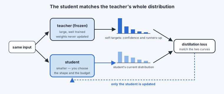
The crucial detail is what the student copies. Ordinary supervised training pushes up the probability of one correct label and says nothing about the rest. The teacher, given the same input, produces a full distribution over the vocabulary — and the shape of that distribution is informative. If the teacher puts most of its mass on one token but meaningful weight on two others, it is telling the student something about which alternatives are reasonable that a single label never could. Training the student against these soft targets consistently beats training it against hard targets (the teacher's top choice, treated as the answer). Hard-target distillation remains useful when the teacher's probabilities are not available, which is often the case behind a commercial API — though copying a hosted model's outputs this way usually breaches its terms of service.
Variations extend the same principle. Rather than match only the final distribution, the student can also be trained to reproduce the teacher's intermediate representations, layer against layer, which supplies a much denser signal. For generation there is a further choice: matching the teacher token by token (word-level), or trying to match it over whole outputs (sequence-level). The latter is the better objective and intractable as written, since it ranges over every possible sequence, so in practice it is approximated by taking the teacher's own best decoded output and training the student to produce that.
What makes distillation expensive is not subtle. Running a large teacher over a large corpus is costly — generation is slow, one token at a time — and then a whole model must be trained on the results. Starting the student from an aggressively pruned copy of the teacher, rather than from scratch, is a common way to shorten that second stage.
Quantization and pruning need no training data; you can compress an open-weights model without ever knowing what it was trained on. Distillation needs data to run the teacher over, and that is the hard part. Labs release weights far more readily than datasets — the data is the asset. In practice this pushes distillation toward task-specific use: you may not be able to reproduce a general assistant, but if you have data for your task, you can distil a small model that handles it well.
The modern inversion: teachers as data factories
There is a second reason very large models are built, beyond serving them directly. A heavily over-parameterised model captures nuances of the data that a smaller one cannot — and once it has, its outputs become training material. Rather than deploy the giant, you use it to manufacture a dataset and train something deployable on that.
The approach that established this pattern started from a small set of hand-written task examples — on the order of a couple of hundred — and prompted a base model, few-shot, to invent new instructions of the same kind, then to produce inputs and outputs for each. Filtering the results leaves a large instruction-tuning dataset grown from a tiny seed. The same recipe is now routine in industry: to build a natural-language interface over an existing system, describe what the system can do, have a strong model synthesise many plausible user phrasings and correct responses, and fine-tune a small model on the result.
Note what changed. Classical distillation can only observe how the teacher reacts to data you already have. A generative teacher can be asked to create the data too. That shift is why synthetic data became central to post-training, and it gets its own lesson later in the course.
Choosing between them
Start with the constraint. If the model nearly fits and you want memory and bandwidth back cheaply, quantize — it is the least invasive and needs no data. If you want more and your hardware rewards a sparsity pattern it supports, prune to that pattern and fine-tune to recover. If you need a large reduction in latency, neither will get you there: only a genuinely smaller architecture will, and that means distillation, with the data and compute bill it brings. They also compose — a distilled student can be pruned and then quantized — and in production systems they usually are.