Bayesian Estimation

Flip a coin three times and get three heads. Maximum likelihood says the coin lands heads with probability 1 and tails are impossible. Nobody actually believes that. You have seen many coins, and nearly all of them are close to fair; three heads in a row happens with a fair coin one time in eight. What you believed before the flips should count for something. Bayesian estimation is the formal way to let it.

The parameter as a random variable

Maximum likelihood treats the unknown parameter $p$ as a fixed number we are trying to pin down. The Bayesian view treats our uncertainty about $p$ as a probability distribution.

• The prior $P(p)$ describes what we believe about $p$ before seeing data.
• The likelihood $P(\text{data} \mid p)$ is the same as before: how probable the observations are for a given $p$.
• Bayes' rule combines them into the posterior $P(p \mid \text{data})$, what we believe after seeing the data:

The denominator does not depend on $p$; it only makes the posterior integrate to 1. So the posterior is the prior, reweighted by how well each value of $p$ explains the data.

A prior for a probability: the Beta distribution

The parameter $p$ lives between 0 and 1, so the prior must too. The standard choice is the Beta distribution with shape parameters $\alpha, \beta > 0$:

where $B(\alpha, \beta)$ is the normalising constant. Different shapes express different beliefs.

• $\text{Beta}(1, 1)$ is flat: every bias equally plausible.
• $\text{Beta}(10, 10)$ peaks at 0.5: "probably close to fair".
• $\text{Beta}(2, 8)$ leans towards small $p$: "probably rarely heads".

Its mean is $\tfrac{\alpha}{\alpha + \beta}$, and the larger $\alpha + \beta$, the more concentrated (confident) it is.

Updating: pseudo-counts

With $k$ heads in $n$ flips, the likelihood is $p^k(1 - p)^{n - k}$. Multiply by the Beta prior:

That is again a Beta distribution:

The update is just addition. The prior behaves as if we had already seen $\alpha - 1$ heads and $\beta - 1$ tails (or, loosely, $\alpha$ and $\beta$ pseudo-counts), and the data adds its real counts. When the prior and posterior belong to the same family like this, the prior is called conjugate to the likelihood. Conjugacy is what makes Bayesian updating a one-line formula here.

From a posterior to a single number

The posterior is a whole distribution, which is its strength: it says how uncertain we still are. When a single estimate is needed, two summaries are common.

• Posterior mean: $\displaystyle \hat p = \frac{\alpha + k}{\alpha + \beta + n}$.
• Posterior mode, the maximum a posteriori (MAP) estimate: $\displaystyle \hat p_{\text{MAP}} = \frac{\alpha + k - 1}{\alpha + \beta + n - 2}$.

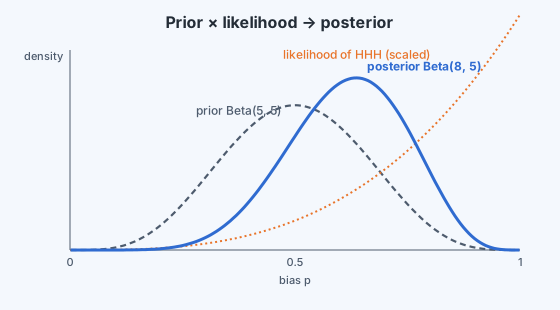
Back to three heads in three flips, with the prior $\text{Beta}(5, 5)$ ("probably near fair"):

• MLE: $3/3 = 1$.
• Posterior: $\text{Beta}(8, 5)$, with mean $8/13 \approx 0.62$ and MAP $7/11 \approx 0.64$.

The data has moved our belief towards heads, but three flips are not enough to overturn a reasonable prior. Now suppose we keep flipping and see 700 heads in 1,000 flips. The posterior is $\text{Beta}(705, 305)$ with mean $705/1010 \approx 0.698$, almost exactly the MLE of 0.7. With plenty of data, the likelihood dominates and the prior hardly matters; with little data, the prior keeps the estimate sensible.

The flat prior $\text{Beta}(1, 1)$ gives a posterior mean of $\tfrac{k + 1}{n + 2}$, known as Laplace's rule of succession: after three heads in three flips it predicts heads with probability $4/5$, not 1. The same "add one to every count" idea will return as Laplace smoothing in naive Bayes.

Maximum likelihood versus Bayesian estimation

The MAP estimate is the bridge between the two. It maximises $\ln P(\text{data} \mid p) + \ln P(p)$: the log-likelihood plus a penalty from the prior. In regression we will see that a Gaussian prior on the weights turns least squares into ridge regression, so regularisation is, in this precise sense, a prior belief that the weights are small.