Binary Classification and k-Nearest Neighbours

Regression predicts a number. Many of the most important prediction problems instead ask a yes-or-no question: is this email spam, will this customer leave, does this scan show a tumour, is this transaction fraudulent? This chapter sets up binary classification and meets its simplest method, one that does not train at all.

The problem

The training data is $\{(x_1, y_1), \dots, (x_n, y_n)\}$ with $x_i \in \mathbb{R}^d$ and labels $y_i \in \{-1, +1\}$ (sometimes written $\{0, 1\}$). We want a classifier $h: \mathbb{R}^d \to \{-1, +1\}$.

The natural measure of quality is how often the classifier is wrong, the 0-1 loss:

the fraction of training mistakes (the training error). As always, what we really care about is the error rate on new data.

Why not just reuse regression?

Two obvious approaches both disappoint.

Minimise the 0-1 loss directly over linear classifiers $h(x) = \operatorname{sign}(w^\top x)$. The loss is a step function of $w$: it is flat almost everywhere and jumps when a point crosses the boundary, so gradients are useless. Worse, finding the linear classifier with the fewest mistakes on data that no line separates perfectly is NP-hard in general. We will need smarter substitutes for the 0-1 loss (Modules 9 to 11 are largely about them).

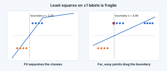
Fit least squares to the labels ±1, then take the sign. It is easy and sometimes acceptable, but it optimises the wrong thing. Squared error punishes predictions that are too correct: a point with label $+1$ and score $+5$ costs $(5 - 1)^2 = 16$, as much as a serious mistake. Add a cluster of easy, far-away points of one class and the regression line tilts towards them to reduce their "error", moving the boundary and creating real mistakes elsewhere.

k-nearest neighbours

k-nearest neighbours (kNN) sidesteps all of this. To classify a new point $x$:

1. Find the $k$ training points closest to $x$ (usually by Euclidean distance).
2. Predict the majority label among them.

There is no training step: the classifier is the stored training set. This is called a non-parametric or instance-based method.

The effect of k

• k = 1 predicts the label of the single nearest training point. Its decision regions are a Voronoi diagram of the training points, the same geometry as k-means, now with one cell per training point. It fits every quirk of the training data, including mislabelled points: a single noisy point carves out an island of the wrong class around itself. Its training error is zero (every point is its own nearest neighbour), which tells you nothing.
• Large k averages over many neighbours, smoothing the boundary and ignoring isolated noise. Too large and it blurs genuine structure away; at $k = n$ every point gets the overall majority class.

So $k$ trades variance (small $k$, sensitive to individual points) against bias (large $k$, too smooth). It is chosen by cross-validation, usually as an odd number to avoid ties between two classes.

Practical issues

• Scale. Distance mixes all features, so a feature measured in large units (income in rupees) swamps one in small units (age in years). Standardise the features first.
• Prediction cost. Every prediction needs the distance to every training point: $O(nd)$ per query, with the whole training set kept in memory. Tree and hashing indexes (k-d trees, approximate nearest-neighbour search, the same vector indexes used in RAG systems) make it practical at scale.
• High dimensions. In many dimensions, distances between random points become nearly equal, so "nearest" carries little information (the curse of dimensionality). kNN works best when the data lies near a low-dimensional structure, or after dimensionality reduction such as PCA.
• No model to inspect. kNN gives predictions but no compact summary of what it learned. In the language of this course, there is no compression at all: the "model" is the data.

That last point motivates the rest of the module. Decision trees, next, keep kNN's flexibility but compress the data into a short list of questions.