PCA and k-means never asked where the data came from. They described its shape directly. This module takes a different stance: assume the data was produced by a random mechanism with some unknown settings, then use the data to work out those settings. That shift, from describing data to modelling how it was generated, is what lets machine learning reason about uncertainty, and it will carry straight over to supervised learning.
A box with a coin inside
Imagine a sealed box with a button. Inside is a coin, not necessarily a fair one: it lands heads with some probability that we do not know. Each press flips the coin and shows us the result, 1 for heads and 0 for tails. After ten presses we see
Two things are now separate.
- What we observe: the ten outcomes.
- What we assume: that a coin with some bias produced them. This is a model, a story we choose in order to explain the data. It may be wrong; it is useful if it is roughly right.
The unknown is called a parameter. Estimation is the job of inferring the parameter from the observations. Notice the compression again: a thousand coin flips are explained by a single number. Once we know , we could build our own box and generate as much data like this as we liked; the data held no information beyond .
Formally, each outcome is a random variable with
a Bernoulli distribution.
Any guess could be right
Seven of the ten flips are heads, so feels like the natural guess. But consider other values.
- Could have produced this data? Certainly: a fair coin gives 7 heads in 10 flips about 12% of the time.
- Could ? Yes, though it would take extraordinary luck.
- Could or ? No. A coin that never lands heads cannot produce a 1, and one that always does cannot produce a 0.
So every value strictly between 0 and 1 remains possible. Once probability enters, we can never be certain of the true parameter. What we need is a principled way to prefer one guess over another, and a principled reason for the intuitive answer 0.7.
The i.i.d. assumption
Two assumptions sit quietly behind the intuitive guess.
- Independent: knowing the outcome of one flip tells us nothing about another. for .
- Identically distributed: every flip uses the same coin, so every has the same distribution, for all .
Together they are called i.i.d.. Two different coins flipped once each would give independent but not identically distributed outcomes.
The likelihood
Under the i.i.d. assumption, the probability of the whole observed sequence factorises into a product. For a coin with bias ,
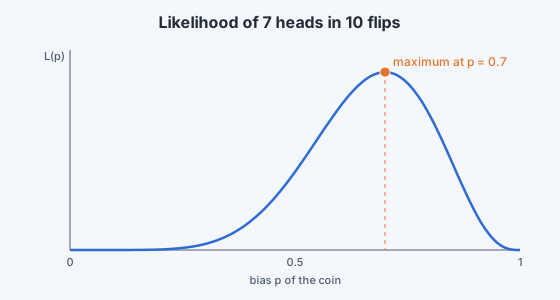
where is the number of heads. Read as a function of the parameter, with the data held fixed, this is the likelihood. It measures how probable our actual observations would be if the parameter were . For our data (, ):
| 0.5 | 0.00098 |
| 0.6 | 0.00179 |
| 0.7 | 0.00222 |
| 0.8 | 0.00168 |
| 0.9 | 0.00048 |
The value makes the data more probable than any of its neighbours.
Maximum likelihood estimation
The maximum likelihood estimate (MLE) is the parameter that makes the observed data most probable:
Products are awkward to differentiate, and the logarithm is increasing, so maximise the log-likelihood instead; it has the same maximiser:
Set the derivative to zero:
The intuitive answer, the fraction of heads, is exactly the maximum likelihood estimate. Now we know why it is a sensible answer, and we have a recipe that works far beyond coins.
The Gaussian case
Many measurements, such as heights, sensor readings and exam marks, are modelled as draws from a Gaussian (normal) distribution with unknown mean and variance :
For i.i.d. observations , the log-likelihood is
Setting the partial derivatives to zero gives
The sample mean and the sample variance (with , not the of many statistics courses). Notice that maximising the likelihood over is the same as minimising the sum of squared distances : the same quantity that k-means minimises within each cluster. This link between Gaussians and squared error will appear again in regression.
How good is the estimate?
The MLE is itself random: a different set of flips gives a different . Two useful properties hold for the coin.
- Unbiased: on average over repeated experiments, .
- Consistent: its variance is , which shrinks as grows, so with enough data the estimate settles on the truth.
The Gaussian variance estimate is slightly biased: its expected value is , because it measures spread around the sample mean, which sits a little closer to the data than the true mean does. Dividing by instead removes the bias; for large the difference is negligible.
The weakness of maximum likelihood shows up with little data. Flip a coin three times, see three heads, and the MLE is : it declares tails impossible. The next chapter fixes this by adding what we believed before seeing the data.