Feature Maps and Kernels

Curved structure becomes linear after mapping each point to a richer feature space, but that space can be astronomically large. A kernel computes the dot product in the feature space directly from the original vectors. Polynomial and RBF kernels are the standard examples, and Mercer's condition tells you which functions are valid kernels.

PCA finds flat structure. This chapter shows how to make curved structure flat, and then how to do so without paying for it. The second half of that sentence is the kernel trick, one of the most reusable ideas in classical machine learning; it will return in regression and in support vector machines.

Curved data, made linear

Take points that lie on a circle of radius $r$ centred at $(a, b)$ . Every point $(f_1, f_2)$ satisfies

(f_1 - a)^2 + (f_2 - b)^2 = r^2 .

PCA cannot see this. After centring, every direction through a circle has about the same spread, so PCA reports two roughly equal eigenvalues and concludes that both dimensions are needed. Yet a circle is a one-dimensional curve: one number (an angle) fixes a point on it.

Expand the equation:

f_1^2 + f_2^2 - 2a\,f_1 - 2b\,f_2 + (a^2 + b^2 - r^2) = 0 .

It is not linear in $(f_1, f_2)$ , but it is linear in the list of terms $(1, f_1, f_2, f_1^2, f_2^2, f_1 f_2)$ . So map each point to

\phi(f_1, f_2) = \big(1,\; f_1,\; f_2,\; f_1^2,\; f_2^2,\; f_1 f_2\big) \in \mathbb{R}^6

and define the fixed vector $u = (a^2 + b^2 - r^2,\; -2a,\; -2b,\; 1,\; 1,\; 0)$ . Then every data point satisfies

u^\top \phi(x) = 0 .

In the six-dimensional feature space, all the mapped points are perpendicular to $u$ : they lie in a linear subspace. Curved structure in the original space has become flat structure in the feature space, which is exactly what PCA can find.

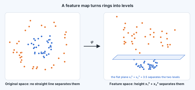
Left: two concentric rings of points in the plane that no straight line separates. Right: the same points lifted into three dimensions with height x1 squared plus x2 squared, where the inner ring sits low and the outer ring high, separated by a flat plane — A feature map φ lifts the data so that curved structure becomes flat. Here adding the feature x₁² + x₂² turns two rings into two levels that a plane can separate.

So the plan is: choose a map $\phi$ that contains the kinds of non-linear terms we expect, map every point, and run PCA in the feature space. Since the feature space has more dimensions than we have points, use the $n \times n$ route from the last chapter.

The cost of the feature space

How big does the feature space get? All terms (monomials) of degree up to $p$ in $d$ variables number

\binom{d + p}{p},

which grows roughly like $d^p / p!$ . Four features with all terms up to degree 3 give $\binom{7}{3} = 35$ coordinates, which is fine. A hundred features up to degree 3 give $176{,}851$ . A thousand features up to degree 2 give over half a million. Computing $\phi(x)$ quickly becomes impractical, and for some useful maps the feature space is infinite-dimensional, so it cannot be computed at all.

Needing only dot products

Recall the observation that ended the last module: the $n \times n$ version of PCA needs only the dot products between points. In the feature space those are

K_{ij} = \phi(x_i)^\top \phi(x_j) .

The coordinates of $\phi(x_i)$ are never used individually. So the question becomes: can we compute $\phi(x)^\top \phi(x')$ without computing $\phi$ ?

A function that computes a dot product in disguise

Take two points in the plane, $x = (f_1, f_2)$ and $x' = (g_1, g_2)$ , and evaluate

k(x, x') = \big(x^\top x' + 1\big)^2 = \big(f_1 g_1 + f_2 g_2 + 1\big)^2 .

Multiply it out:

k(x, x') = f_1^2 g_1^2 + f_2^2 g_2^2 + 2 f_1 g_1 f_2 g_2 + 2 f_1 g_1 + 2 f_2 g_2 + 1 .

Each term is a product of something that depends only on $x$ and the matching thing for $x'$ . Collect them:

k(x, x') = \phi(x)^\top \phi(x'), \qquad \phi(x) = \big(1,\; \sqrt2 f_1,\; \sqrt2 f_2,\; f_1^2,\; f_2^2,\; \sqrt2 f_1 f_2\big).

So one dot product in two dimensions, plus one, squared, gives exactly the dot product of the six-dimensional feature vectors, and that $\phi$ contains every term up to degree two (the $\sqrt 2$ factors just weight them). We computed a six-dimensional dot product without building a single six-dimensional vector.

Kernels

A function $k(x, x')$ is a kernel if there is some map $\phi$ , to some feature space, with

k(x, x') = \phi(x)^\top \phi(x') \quad \text{for all } x, x' .

Two families do most of the work in practice.

Polynomial kernel: $k(x, x') = (x^\top x' + 1)^p$ . Its feature space holds every monomial up to degree $p$ (weighted by binomial coefficients), $\binom{d+p}{p}$ dimensions in all, yet each evaluation costs one $d$ -dimensional dot product.
Radial basis function (RBF), or Gaussian, kernel: $k(x, x') = \exp\!\big(-\lVert x - x' \rVert^2 / 2\sigma^2\big)$ . Its feature space is infinite-dimensional: expanding the exponential as a power series produces terms of every degree, with decreasing weights. It measures similarity by distance: nearly 1 for close points, nearly 0 for far ones, with $\sigma$ setting what counts as close.

Which functions are kernels?

Not every function of two points is a dot product somewhere. One way to prove a function is a kernel is to exhibit $\phi$ , as we did above. When that is hard, Mercer's theorem gives a test. Informally, $k$ is a valid kernel if and only if:

it is symmetric: $k(x, x') = k(x', x)$ ; and
for every finite set of points $x_1, \dots, x_n$ , the matrix $K_{ij} = k(x_i, x_j)$ is positive semi-definite (all its eigenvalues are $\ge 0$ ).

The necessity of both conditions is easy to see. Dot products are symmetric, so $k$ must be. And if $K_{ij} = \phi(x_i)^\top\phi(x_j)$ , then $K = \Phi^\top\Phi$ for the matrix $\Phi$ of mapped points, whose non-zero eigenvalues are those of the (scaled) covariance matrix in the feature space, which are variances and hence non-negative. The deep part of the theorem is that these conditions are also sufficient: any symmetric function whose matrices are always positive semi-definite is a dot product in some feature space.

Mercer's condition also gives a quick way to disprove a candidate. If you can find a single small set of points whose kernel matrix has a negative eigenvalue, the function is not a kernel.

Try it yourself

Machine Learning Lab: feature maps →

Switch between no feature map, adding x₁² + x₂², and all degree-2 terms (exactly the feature space of the quadratic kernel). Watch the rings separate along a single principal component.

MediumKernels

Verify that k(x, x') = (xᵀx')² is a kernel for points in the plane by finding its feature map.

HardKernelsMercer

Is k(x, x') = ‖x − x'‖² a valid kernel?

MediumKernelsRBF