Gaussian Mixture Models

A Gaussian mixture model explains multimodal data with a generative story: pick a component with probability π_k, then draw from that component's Gaussian. The hidden component choice is a latent variable. Summing it out gives a log-likelihood with a log of a sum, which has no closed-form maximiser, so a new algorithm is needed.

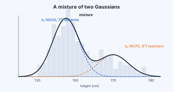
Suppose you record the heights of everyone in a school: students and teachers. Plot a histogram and you see two humps, one around the typical student height and one around the typical adult height. A single Gaussian, with one peak, describes this badly: its maximum likelihood fit puts the peak in the valley between the humps, where hardly anyone is. The data is multimodal, and we need a model that can have several peaks. The Gaussian mixture model (GMM) is the standard answer, and it is also a probabilistic version of clustering.

The generative story

A GMM with $K$ components explains each data point by a two-step random process.

Choose a component. Pick $z \in \{1, \dots, K\}$ at random, with $P(z = k) = \pi_k$ . The mixing proportions $\pi_1, \dots, \pi_K$ are non-negative and sum to 1.
Draw from that component. Given $z = k$ , draw $x$ from a Gaussian with mean $\mu_k$ and variance $\sigma_k^2$ (in $d$ dimensions, mean vector $\mu_k$ and covariance matrix $\Sigma_k$ ).

For the school, $K = 2$ : component 1 is "student", component 2 is "teacher", and $\pi_1$ is the fraction of students. Each component has its own centre and its own spread, unlike k-means, where every cluster is described by a centre alone.

The parameters to estimate are

\theta = \{\pi_1, \dots, \pi_K,\; \mu_1, \dots, \mu_K,\; \sigma^2_1, \dots, \sigma^2_K\},

which is $3K - 1$ numbers in one dimension (the $\pi_k$ must sum to 1).

A histogram of heights with two humps; two weighted Gaussian curves, one for each component, and their sum tracing the two-humped shape — A two-component Gaussian mixture. Each component is a weighted Gaussian (π_k times its bell curve); their sum is the mixture density, which can have several peaks.

Latent variables

We observe the heights $x_1, \dots, x_n$ but not which component produced each one: nobody wrote "student" or "teacher" next to the measurements. The component choices $z_1, \dots, z_n$ are latent (hidden) variables. They are exactly the cluster indicators of k-means, except that now they are random, and we will reason about their probabilities instead of assigning them outright.

The mixture density

The probability density of a single observation is found by summing over the component it might have come from:

f(x;\theta) = \sum_{k=1}^{K} P(z = k)\, f(x \mid z = k) = \sum_{k=1}^{K} \pi_k\, \mathcal{N}(x;\, \mu_k, \sigma_k^2),

where $\mathcal{N}(x; \mu, \sigma^2)$ is the Gaussian density. It is a weighted average of $K$ bell curves, which can have up to $K$ peaks and many other shapes. With enough components, a Gaussian mixture can approximate essentially any smooth density, which makes it a general-purpose tool for density estimation as well as clustering.

The log-likelihood, and why it is hard

With i.i.d. data, the log-likelihood is

\ell(\theta) = \sum_{i=1}^{n} \ln\Big( \sum_{k=1}^{K} \pi_k\, \mathcal{N}(x_i;\, \mu_k, \sigma_k^2) \Big).

Compare it with a single Gaussian. There the log could pass through to the exponent, the log-likelihood became a simple quadratic in $\mu$ , and setting its derivative to zero gave the answer in one line. Here the log sits outside a sum, and the derivative with respect to $\mu_k$ becomes

\frac{\partial \ell}{\partial \mu_k} = \sum_{i=1}^{n} \underbrace{\frac{\pi_k \mathcal{N}(x_i; \mu_k, \sigma_k^2)}{\sum_{j} \pi_j \mathcal{N}(x_i; \mu_j, \sigma_j^2)}}_{\text{depends on all the parameters}} \cdot \frac{x_i - \mu_k}{\sigma_k^2} .

Setting it to zero does not give a closed-form solution: the weights in front of each term depend on every parameter, including $\mu_k$ itself. There is no formula for the maximum likelihood estimate of a GMM.

There are further complications. The log-likelihood is not concave, so it can have several local maxima. Swapping the labels of two components gives the same likelihood, so the maxima come in groups of $K!$ equivalent solutions. And if one component shrinks onto a single data point ( $\mu_k = x_i$ , $\sigma_k \to 0$ ), its density at that point grows without bound, so the likelihood itself is unbounded: an unconstrained maximum likelihood fit can "cheat" by collapsing a component. In practice a small floor on the variances prevents this.

A clue in the derivative

Look again at the weight in the derivative above:

\lambda_{ik} = \frac{\pi_k\, \mathcal{N}(x_i;\mu_k,\sigma_k^2)}{\sum_{j}\pi_j\, \mathcal{N}(x_i;\mu_j,\sigma_j^2)} .

By Bayes' rule, this is exactly $P(z_i = k \mid x_i)$ : the probability that point $i$ came from component $k$ , given its value. It is called the responsibility of component $k$ for point $i$ . If we knew the responsibilities, setting the derivative to zero would give a simple weighted mean:

\mu_k = \frac{\sum_i \lambda_{ik}\, x_i}{\sum_i \lambda_{ik}} .

And if we knew the parameters, computing the responsibilities would be easy. This chicken-and-egg structure is the same one k-means had (assignments need centres, centres need assignments), and it suggests the same remedy: alternate. The next chapter turns that idea into the EM algorithm and shows why it works.

Try it yourself

Machine Learning Lab: Gaussian mixtures →

See three Gaussian components fitted to two-dimensional data, with every point coloured by its responsibilities: mixed colours mark the points that lie between components.

MediumGMMBayes rule

A 1-D mixture has π = (0.3, 0.7), means 0 and 5, and both variances 1. What is the probability that the point x = 2 came from the first component?

MediumGMMModel selection

How many parameters does a K-component Gaussian mixture have in d dimensions with full covariance matrices?

HardGMMMLE