Gaussian Naive Bayes

For real-valued features, model each feature within each class as a Gaussian and estimate its mean and variance by maximum likelihood. Classifying by the larger posterior gives a quadratic boundary in general; when the classes share their variances the quadratic terms cancel and the boundary is linear, the same family as logistic regression.

Naive Bayes on words used coin-flip features: a word is present or not. Many problems have real-valued features instead: a flower's petal length, a patient's blood pressure, a sensor's temperature. The generative recipe still applies; only the model of each feature changes. The obvious choice for a continuous measurement is a Gaussian.

The model

For a binary problem with features $x \in \mathbb{R}^d$ :

The class prior is $P(y = 1) = p$ .
Within class $y$ , feature $j$ is Gaussian with its own mean and variance: $x_j \mid y \sim \mathcal{N}(\mu_{yj}, \sigma^2_{yj})$ .
The naive assumption: within a class, the features are independent, so $P(x \mid y) = \prod_{j=1}^{d} \mathcal{N}(x_j;\, \mu_{yj}, \sigma^2_{yj}) .$

Geometrically, each class is modelled as an axis-aligned Gaussian blob: an ellipse whose axes are parallel to the feature axes, because independence means no correlation between features within a class.

Training

Each parameter has the maximum likelihood estimate from Module 5, computed on that class's points only:

\hat p = \frac{n_1}{n}, \qquad \hat\mu_{yj} = \frac{1}{n_y}\sum_{i:\,y_i = y} x_{ij}, \qquad \hat\sigma^2_{yj} = \frac{1}{n_y}\sum_{i:\,y_i = y}\big(x_{ij} - \hat\mu_{yj}\big)^2 ,

where $n_y$ is the number of training points in class $y$ . Training is again a single pass: per class and per feature, a mean and a variance. (A small constant is usually added to each variance so that a feature that happens to be constant within a class does not get variance zero.)

Classifying, and the shape of the boundary

Compare the log posteriors. For class $y$ ,

\text{score}_y(x) = \ln P(y) - \sum_{j=1}^{d}\Big[\frac{(x_j - \mu_{yj})^2}{2\sigma^2_{yj}} + \ln\sigma_{yj}\Big] + \text{const}.

Predict class 1 when $\text{score}_1(x) > \text{score}_0(x)$ . The boundary is where the two scores are equal. Each score contains terms in $x_j^2$ with coefficient $-1/(2\sigma^2_{yj})$ , so in general:

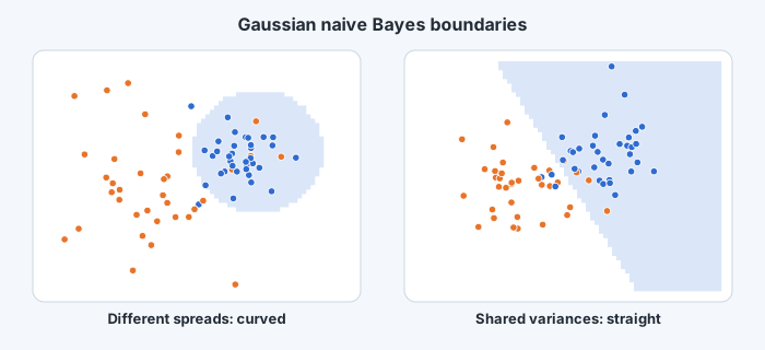
The boundary is quadratic. If the two classes have different variances for a feature, the $x_j^2$ terms do not cancel, and the boundary is a curve: an ellipse, a parabola or a hyperbola in two dimensions. A tight class surrounded by a widely spread one gets a closed boundary around it.

With shared variances, the boundary is linear. If $\sigma^2_{1j} = \sigma^2_{0j} = \sigma^2_j$ for every feature, the $x_j^2$ terms are identical in both scores and cancel, leaving

\sum_{j=1}^{d}\frac{\mu_{1j} - \mu_{0j}}{\sigma^2_j}\,x_j \;+\; b \;>\; 0 ,

a linear classifier, with each feature weighted by how far apart the class means are relative to that feature's spread. This is the same family as logistic regression, and the same family as naive Bayes on binary features.

Two panels. Left: a tight blue class and a wide orange class, each with an axis-aligned elliptical contour, and a curved decision boundary wrapping around the blue class. Right: two classes with the same spread and a straight decision boundary between them — Gaussian naive Bayes. With different spreads per class the boundary curves (left); with shared variances it is a straight line (right).

Try it yourself

Machine Learning Lab: naive Bayes vs logistic →

Widen the orange class and watch the naive Bayes boundary curl around the blue one. Tick "share variances" and it straightens into a line, close to logistic regression's.

Generative classifiers, compared

Naive Bayes is the simplest member of a family of Gaussian generative classifiers. They differ only in how much structure the class covariance matrices may have.

Model	Class covariance	Boundary
Gaussian naive Bayes, shared variances	diagonal, the same for both classes	linear
Gaussian naive Bayes	diagonal, per class	quadratic
Linear discriminant analysis (LDA)	full, shared	linear
Quadratic discriminant analysis (QDA)	full, per class	quadratic

More freedom means more parameters to estimate (a full covariance matrix has $d(d+1)/2$ entries), so the richer models need more data. Naive Bayes sits at the cheap end: it ignores correlations between features, and in return needs only $2d$ numbers per class.

When the assumptions fail

Gaussian naive Bayes is fast, needs little data and gives sensible probabilities when its assumptions roughly hold. Two failures are common.

Non-Gaussian features. A feature with two peaks within a class, or heavy skew, is poorly described by one Gaussian. Transforming the feature (a logarithm for skewed positive quantities) or using a mixture per class helps.
Strongly correlated features. Independence counts correlated evidence twice. The predicted class may still be right, but the probabilities become overconfident, pushed towards 0 and 1.

In both cases a discriminative method such as logistic regression, which makes no assumption about how the features are distributed, is a natural alternative, and it is the next chapter's subject.

EasyGaussian naive Bayes

A one-feature problem: class 0 has mean 0, class 1 has mean 4, both with variance 1 and equal priors. Where is the decision boundary?

HardGaussian naive BayesQuadratic boundary

Same means 0 and 4, but class 1 now has variance 4 (class 0 still 1), equal priors. Show the boundary is not a single point.

MediumNaive BayesAssumptions