The Geometry of Least Squares and Gradient Descent

The least-squares formula $w^* = (XX^\top)^{-1}Xy$ came out of setting a gradient to zero. This chapter looks at it twice more: once as geometry, which explains what least squares is doing, and once as an algorithm, which explains how to compute it when the formula is too expensive.

Least squares is a projection

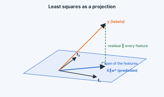
Change the point of view. Instead of $n$ points in $d$-dimensional feature space, think of $n$-dimensional vectors, one entry per training example.

• The labels form one vector $y \in \mathbb{R}^n$.
• Each feature also forms a vector in $\mathbb{R}^n$: its values across the $n$ examples. These are the rows of $X$, or the columns of $X^\top$.
• Any prediction vector $X^\top w = \sum_j w_j\,(\text{feature } j)$ is a linear combination of the feature vectors. As $w$ varies, the predictions sweep out the column space of $X^\top$, a subspace of $\mathbb{R}^n$ of dimension at most $d$.

Least squares picks the point of that subspace closest to $y$:

The closest point of a subspace to a vector is its orthogonal projection, the same idea as finding a proxy in PCA, now in $\mathbb{R}^n$. At the projection, the residual $r = y - X^\top w^*$ is perpendicular to the whole subspace, which means perpendicular to every feature vector:

These are exactly the normal equations. The algebra and the geometry agree: least squares projects the labels onto the span of the features, and whatever part of $y$ cannot be expressed through the features is left over as a residual orthogonal to all of them.

Two useful consequences follow.

• If a feature is the constant 1 (the intercept), the residual is orthogonal to the all-ones vector, so the residuals sum to zero: the fitted line passes through the mean of the data.
• Adding a feature can only enlarge the subspace, so the training error can only fall or stay the same. That is why training error alone can never tell you to stop adding features.

When the formula is too expensive

Computing $w^*$ directly means forming the $d \times d$ matrix $XX^\top$ (about $nd^2$ operations) and solving a $d \times d$ system (about $d^3$). With millions of features, or data too large to hold in memory, that is impractical. The alternative is to approach the minimum step by step.

Gradient descent

The gradient of the loss points in the direction of steepest increase. Take a small step the other way, and repeat:

where $\eta > 0$ is the learning rate (step size). Each step costs one pass over the data, about $nd$ operations, and needs no matrix inverse. Because the squared-error loss is a convex bowl, gradient descent with a small enough $\eta$ converges to the global minimum.

The step size matters.

• Too small: progress is slow; thousands of steps to cross a gentle slope.
• Too large: the steps overshoot the bottom of the bowl and can grow without limit (for least squares, divergence starts once $\eta$ exceeds $1/\lambda_{\max}(XX^\top)$, where $\lambda_{\max}$ is the largest eigenvalue).
• A long, narrow bowl (features on very different scales) makes gradient descent zigzag. Standardising the features (zero mean, unit variance) rounds the bowl and speeds it up.

Stochastic gradient descent

The full gradient is a sum over all $n$ points. Stochastic gradient descent (SGD) estimates it from a single randomly chosen point, or a small random mini-batch $B$:

The estimate is noisy but correct on average (unbiased), and each step is cheap: it touches $|B|$ points instead of $n$. In the time one full-gradient step takes, SGD makes $n/|B|$ steps, which usually wins by a wide margin on large data. The noise means SGD does not settle exactly at the minimum with a fixed step size; it hovers around it. Shrinking $\eta$ over time, or averaging the recent iterates, brings it home. This is the same algorithm that trains neural networks, where no closed form exists at all.