Kernel PCA

We now have every ingredient. PCA can be computed from an $n \times n$ matrix of dot products, and a kernel supplies dot products in a feature space we never have to construct. Putting the two together gives kernel PCA: non-linear dimensionality reduction at the cost of an $n \times n$ eigen-decomposition.

The algorithm, first draft

Input: data $x_1, \dots, x_n \in \mathbb{R}^d$ and a valid kernel $k$.

1. Build the kernel matrix $K \in \mathbb{R}^{n \times n}$ with $K_{ij} = k(x_i, x_j)$.
2. Eigen-decompose it: unit eigenvectors $\beta_1, \beta_2, \dots$ with eigenvalues $n\lambda_1 \ge n\lambda_2 \ge \dots$
3. Rescale: $\alpha_k = \beta_k / \sqrt{n\lambda_k}$.

In ordinary PCA the next step was $w_k = X\alpha_k$. Here the same step would read

and that needs $\phi$, which we are not allowed to compute (for the RBF kernel it is infinite-dimensional). So we cannot write down the principal directions in the feature space.

We never needed the directions

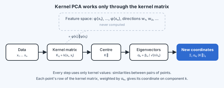
What do we actually use PCA for? Usually not for the directions themselves, but for each point's coordinates along them: the compressed representation. The coordinate of point $x_i$ on the $k$-th direction is

Only kernel values appear. So each point's new representation is

Read it this way: row $i$ of $K$ lists how similar $x_i$ is to every training point, and each component weights those similarities in its own way. A new point $x$ is handled the same way, using the similarities $k(x, x_j)$ to the training points.

What we give up is reconstruction. Turning coefficients back into a point needs the directions $w_k$, which live in the feature space. For most uses (visualisation, clustering, or feeding a classifier) the coordinates are what matter, and we have them.

Note that $\ell$ can exceed the original $d$. With two-dimensional data and an RBF kernel you might keep ten components. That is not a contradiction: the data has been lifted to a much larger space where its curved structure is flat, and ten coordinates in that space can describe it far better than the original two.

The missing step: centring in feature space

Ordinary PCA centred the data first. Kernel PCA needs the mapped points $\phi(x_i)$ centred, but we cannot subtract their mean $\mu_\phi = \tfrac1n\sum_i \phi(x_i)$ because we cannot compute any of them. Fortunately the dot products of the centred points can be written using only kernel values:

Each term comes from expanding the product: the original kernel value, minus the average similarity of $x_i$ to all points, minus that of $x_j$, plus the overall average. In matrix form, with $\mathbf{1}_n$ the $n \times n$ matrix whose every entry is $1/n$,

Use $K_c$ in place of $K$ from step 2 onwards.

Kernel PCA, complete

1. Compute $K_{ij} = k(x_i, x_j)$.
2. Centre it: $K_c = K - \mathbf{1}_n K - K\mathbf{1}_n + \mathbf{1}_n K \mathbf{1}_n$.
3. Eigen-decompose $K_c$: unit eigenvectors $\beta_k$, eigenvalues $n\lambda_k$, largest first.
4. Rescale: $\alpha_k = \beta_k / \sqrt{n\lambda_k}$.
5. Represent each training point by its $\ell$ coordinates $\sum_j \alpha_{k,j} (K_c)_{ij}$, for $k = 1, \dots, \ell$.

Choosing the kernel

The kernel decides what structure kernel PCA can find. A polynomial kernel of degree 2 can flatten circles, ellipses and parabolas; higher degrees capture more intricate surfaces. The RBF kernel can follow almost any smooth shape, with $\sigma$ controlling how local it is: a small $\sigma$ makes every point similar only to its immediate neighbours (very flexible, prone to fitting noise), a large $\sigma$ makes the kernel behave almost linearly. With a linear kernel, $k(x, x') = x^\top x'$, kernel PCA is exactly ordinary PCA.

The bigger lesson

Look at how kernel PCA came about. We solved the problem for linear structure, noticed the solution needed only dot products between data points, and swapped those dot products for a kernel. That recipe, solve it linearly, check that only dot products appear, then kernelise, is general. We will apply it again to regression in Module 6 and to support vector machines in Module 10.