Kernel Regression

Kernel PCA came from one observation: if an algorithm needs only dot products between data points, a kernel can replace them and the algorithm becomes non-linear for free. Linear regression passes the same test, and the result, kernel regression, can fit curves of almost any shape while still solving a linear system.

The weights live in the span of the data

The least-squares solution satisfies the normal equations $XX^\top w^* = Xy$. Look at the right-hand side: $Xy = \sum_i y_i x_i$ is a combination of the training points. A short argument shows that the solution can always be taken as such a combination too. Split any weight vector into a part inside the span of the training points and a part orthogonal to all of them: $w = X\alpha + w_\perp$. The orthogonal part has $x_i^\top w_\perp = 0$ for every training point, so it changes no training prediction and cannot reduce the loss; dropping it loses nothing. Hence there is an optimal solution of the form

This is the regression version of the fact we used in kernel PCA, that the principal components are combinations of the data points, and it is a simple case of a general result called the representer theorem.

Everything in terms of dot products

Substitute $w = X\alpha$.

Predictions on the training set are $X^\top w = X^\top X\alpha = K\alpha$, where $K = X^\top X$ is the $n \times n$ matrix of dot products, $K_{ij} = x_i^\top x_j$. The loss becomes

which is minimised when $K\alpha = y$, so (if $K$ is invertible) $\alpha^* = K^{-1}y$.

A prediction for a new point $x$ is

Again only dot products appear: between the new point and each training point.

Swapping in a kernel

Replace every dot product $x_i^\top x_j$ by a kernel $k(x_i, x_j)$, which computes a dot product $\phi(x_i)^\top\phi(x_j)$ in some feature space:

This is linear regression in the feature space of $\phi$, carried out without ever computing $\phi$. With a polynomial kernel of degree $p$ it fits polynomials of degree $p$; with the RBF kernel it fits smooth curves of essentially any shape.

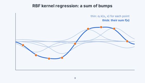
The prediction has an appealing reading. Each training point $x_i$ places a bump $\alpha_i\,k(x_i, \cdot)$ centred on itself, and the prediction at $x$ is the sum of all the bumps there. With the RBF kernel, nearby training points dominate and distant ones contribute almost nothing: the model predicts by similarity to the examples it has seen.

Making it work in practice: add a ridge

Solving $K\alpha = y$ exactly makes the curve pass through every training point, noise included, which is overfitting in its purest form. With the RBF kernel, $K$ is also often nearly singular (two close points give two nearly identical rows), so $K^{-1}$ is numerically unstable. The standard remedy adds a small multiple of the identity:

This is kernel ridge regression. The term $\lambda I$ makes the system well conditioned and stops the fit from chasing every noisy label; the next chapters show that it corresponds to a penalty on the size of the weights (equivalently, a prior belief that they are small). Choosing $\lambda$, and the kernel's own parameters such as the RBF width $\sigma$, is done by validation.

The cost of kernels

Kernel regression trades the $d \times d$ system of ordinary least squares for an $n \times n$ one: about $n^3$ operations to solve and $n^2$ numbers to store. Prediction needs every training point (all $n$ kernel values for each new $x$), unlike linear regression, which only needs $w$. That is fine for thousands of points and painful for millions. Approximations such as random features or using a subset of points as centres keep kernel methods practical at scale. Support vector machines (Module 10) solve the prediction-cost problem differently: their solution keeps only a few training points.