Linear Regression and Least Squares

Supervised learning adds a label to each point. Regression predicts a real-valued label with a function chosen from a family; linear regression uses w·x and scores it by squared error. Setting the gradient of the squared error to zero gives the normal equations and the closed form w* = (XXᵀ)⁻¹Xy. Low training error alone can mean overfitting.

Everything so far has been unsupervised: data points with no answers attached. From here the course turns to supervised learning, where every training point comes with a label, the answer we want to predict. This chapter starts with the simplest supervised problem and the most widely used model of all: predicting a number with a straight line.

The supervised set-up

The training data is a set of pairs

\{(x_1, y_1), (x_2, y_2), \dots, (x_n, y_n)\}, \qquad x_i \in \mathbb{R}^d .

The features $x_i$ describe an example; the label $y_i$ is the answer.

In regression the label is a real number: $y_i \in \mathbb{R}$ . A house's floor area, age and distance to the station ( $x$ ) and its price ( $y$ ).
In classification the label is a category: $y_i \in \{-1, +1\}$ for two classes, or one of $K$ classes. Modules 7 to 10 cover classification.

The goal is a function $h: \mathbb{R}^d \to \mathbb{R}$ , learned from the training pairs, that predicts the label of a new $x$ well. As in Module 1, success means doing well on data the model has not seen.

Choosing a family and a loss

Searching over all possible functions is hopeless (and any function that simply memorises the training pairs would fit them perfectly). We restrict the search to a family, and the simplest useful family is the linear functions:

h_w(x) = w^\top x = w_1 x_1 + w_2 x_2 + \dots + w_d x_d .

The weights $w$ are the parameters to learn. To include an intercept (a value when every feature is zero), append a constant feature $x_0 = 1$ ; its weight plays the role of the intercept, so we can keep writing $w^\top x$ .

To compare weight vectors we need a loss, a measure of how wrong the predictions are. The standard choice is the squared error, summed over the training set:

L(w) = \sum_{i=1}^{n} \big(w^\top x_i - y_i\big)^2 .

Squaring makes every error count positively, punishes large errors far more than small ones, and (as we will see) produces a smooth bowl-shaped function with a single minimum. Finding the $w$ that minimises it is least squares.

Solving it

Stack the training points as the columns of $X \in \mathbb{R}^{d \times n}$ (as we did for PCA) and the labels into $y \in \mathbb{R}^n$ . The predictions for all points at once are $X^\top w$ , so

L(w) = \lVert X^\top w - y \rVert^2 .

Its gradient is

\nabla L(w) = 2X\big(X^\top w - y\big) .

Setting it to zero gives the normal equations

X X^\top w = X y ,

and, when $XX^\top$ is invertible,

w^* = \big(XX^\top\big)^{-1} X y .

$L$ is a convex quadratic (its Hessian $2XX^\top$ is positive semi-definite), so this stationary point is the global minimum. The matrix $XX^\top$ is $d \times d$ , the same matrix that appeared, divided by $n$ , as the covariance matrix in PCA.

A small example

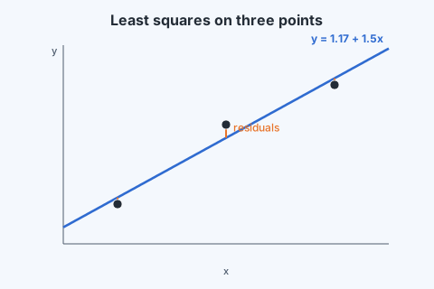
Fit $y \approx w_0 + w_1 x$ to three points: $(0, 1), (1, 3), (2, 4)$ . With the constant feature, each $x_i = (1, x_i)$ :

XX^\top = \begin{bmatrix} 3 & 3 \\ 3 & 5 \end{bmatrix}, \qquad Xy = \begin{bmatrix} 8 \\ 11 \end{bmatrix}, \qquad w^* = \frac{1}{6}\begin{bmatrix} 5 & -3 \\ -3 & 3 \end{bmatrix}\begin{bmatrix} 8 \\ 11 \end{bmatrix} = \begin{bmatrix} 7/6 \\ 3/2 \end{bmatrix}.

The line is $y = 1.17 + 1.5x$ . Its predictions $1.17, 2.67, 4.17$ miss the labels by $0.17, -0.33, 0.17$ , and no other line has a smaller sum of squared misses ( $1/6$ ).

Three points and the least-squares line through them, with vertical segments from each point to the line showing the residuals that are squared and summed — Least squares chooses the line that minimises the sum of squared vertical gaps (residuals) between the labels and the predictions.

Non-linear features, still linear regression

"Linear" refers to the weights, not to the shape of the curve. Replace $x$ by any fixed set of features, such as $(1, x, x^2, x^3)$ , and the model $w_0 + w_1x + w_2x^2 + w_3x^3$ is still linear in $w$ . The same formula $w^* = (\Phi\Phi^\top)^{-1}\Phi y$ fits it, with the feature matrix $\Phi$ in place of $X$ . Polynomial regression, regression on logarithms or on products of features: all are linear regression on transformed features, the same feature-map idea we met in kernel PCA.

Fitting the training data is not the goal

With features $1, x, \dots, x^{n-1}$ , a polynomial can pass through all $n$ training points exactly: zero training error. But between the points such a curve swings wildly, and its predictions on new points are poor. This is overfitting: the model has fitted the noise in the training labels rather than the underlying pattern. A model that is too rigid has the opposite problem, underfitting: a straight line through a wavy pattern is wrong everywhere.

What we really want is low generalisation error, the expected error on new data from the same source. Training error is an optimistic estimate of it, increasingly so as the model becomes more flexible. Later chapters give the tools to control this: held-out validation data (cross-validation), and penalties on the size of the weights (ridge and lasso).

Try it yourself

Machine Learning Lab: regression →

Raise the polynomial degree from 1 to 12 and watch training error keep falling while the error on new points falls and then shoots up.

EasyLeast squares

Fit y ≈ w x (no intercept) by least squares to the points (1, 2), (2, 3), (3, 7).

MediumLeast squaresLinear algebra

When is XXᵀ not invertible, and what does that mean for least squares?

EasyOverfitting