Logistic Regression

Logistic regression models P(y = 1 | x) as the sigmoid of w·x, so the score's sign gives the class and its size the confidence. Maximum likelihood gives the cross-entropy (log) loss, which is convex but has no closed-form minimiser; gradient descent uses the gradient Σ(σ(w·xᵢ) − yᵢ)xᵢ. On separable data the weights grow without bound unless regularised.

The perceptron gives a hard answer: $+1$ or $-1$ , with no sense of how sure it is. Often we need more. A bank approving loans, a doctor triaging patients and an advertiser bidding for clicks all need the probability of each outcome, not just a guess. Logistic regression is the standard discriminative way to get one. Despite its name, it is a classification method.

From a score to a probability

Keep the linear score $z = w^\top x$ and turn it into a probability with the sigmoid (logistic) function:

\sigma(z) = \frac{1}{1 + e^{-z}} .

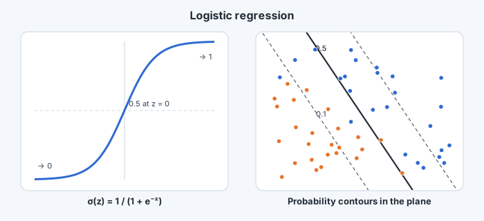
It squashes any real number into $(0, 1)$ : $\sigma(0) = 0.5$ , large positive scores approach 1, large negative scores approach 0, and $\sigma(-z) = 1 - \sigma(z)$ . The model is

P(y = 1 \mid x) = \sigma(w^\top x), \qquad P(y = 0 \mid x) = 1 - \sigma(w^\top x).

The decision boundary, where the probability is exactly 0.5, is $w^\top x = 0$ : still a hyperplane. What logistic regression adds is a graded confidence that rises smoothly as a point moves away from the boundary in the direction of $w$ .

Turned around, the score is the log-odds of class 1:

\ln\frac{P(y = 1 \mid x)}{P(y = 0 \mid x)} = w^\top x .

Each weight therefore has a clean meaning: raising feature $j$ by one unit adds $w_j$ to the log-odds, multiplying the odds by $e^{w_j}$ . This interpretability is a large part of why logistic regression dominates medicine, economics and credit scoring.

Try it yourself

Deep Learning Lab: sigmoid versus step →

Compare the perceptron's hard step with the smooth sigmoid, and see how the weights stretch and shift the curve.

Fitting by maximum likelihood

With labels $y_i \in \{0, 1\}$ , each label is a Bernoulli draw with probability $p_i = \sigma(w^\top x_i)$ . The likelihood of all the labels is

L(w) = \prod_{i=1}^{n} p_i^{\,y_i}(1 - p_i)^{1 - y_i},

and the negative log-likelihood, the quantity to minimise, is the cross-entropy (or log) loss:

\mathcal{L}(w) = -\sum_{i=1}^{n}\Big[y_i \ln \sigma(w^\top x_i) + (1 - y_i)\ln\big(1 - \sigma(w^\top x_i)\big)\Big].

It charges a point little when the model gives its true label a high probability, and a great deal when the model is confidently wrong: predicting 0.01 for a point whose label is 1 costs $-\ln 0.01 \approx 4.6$ .

The gradient

The sigmoid has a convenient derivative, $\sigma'(z) = \sigma(z)\,(1 - \sigma(z))$ . Using it, the gradient of the loss simplifies to

\nabla \mathcal{L}(w) = \sum_{i=1}^{n}\big(\sigma(w^\top x_i) - y_i\big)\, x_i .

Each point contributes its prediction error (predicted probability minus true label) times its features: the same form as the least-squares gradient, with the sigmoid in place of the identity. Setting it to zero has no closed-form solution, because $w$ sits inside a non-linear function. But the loss is convex (its Hessian $\sum_i \sigma_i(1 - \sigma_i)\,x_ix_i^\top$ is positive semi-definite), so it has no misleading local minima: gradient descent, SGD or Newton's method all reach the global minimum.

w \;\leftarrow\; w - \eta \sum_{i=1}^{n}\big(\sigma(w^\top x_i) - y_i\big)\,x_i .

Compare with the perceptron: it updates only on mistakes and by the full $y_i x_i$ . Logistic regression updates on every point, by an amount proportional to how wrong its probability is, so points that are correct but unconvincing still nudge the boundary.

Left: the S-shaped sigmoid curve from 0 to 1, crossing 0.5 at a score of zero. Right: two classes of points in the plane with the logistic regression boundary and parallel contour lines of predicted probability 0.1, 0.5 and 0.9 — Logistic regression. The sigmoid turns a linear score into a probability (left); in the feature plane the 0.5 contour is the boundary and probability changes smoothly across it (right).

A trap: separable data

If the training data is linearly separable, the likelihood can be pushed ever closer to 1 by scaling up $w$ : doubling $w$ keeps the boundary but makes every probability more extreme, and correct, so the loss keeps falling towards zero. Gradient descent then never converges; the weights grow without bound and the model becomes absurdly confident.

The cure is regularisation, exactly as in ridge regression: minimise

\mathcal{L}(w) + \lambda\lVert w\rVert^2 ,

which is the MAP estimate under a Gaussian prior on $w$ . It keeps the weights finite, makes the probabilities more realistic, and helps generalisation even when the data is not separable. Most software applies such a penalty by default.

Beyond two classes

For $K$ classes, give each class its own weight vector and replace the sigmoid by the softmax:

P(y = k \mid x) = \frac{e^{w_k^\top x}}{\sum_{j=1}^{K} e^{w_j^\top x}} .

This is multinomial logistic regression (softmax regression), fitted with the same cross-entropy loss. It is also exactly the final layer of most neural network classifiers, including the next-token layer of a language model.

EasyLogistic regression

A logistic regression model has weights w = (−3, 0.8) with features (1, hours studied). What is the predicted probability of passing after 5 hours, and how do the odds change per extra hour?

MediumLogistic regressionGradient

Derive the logistic regression gradient for one point.

MediumLogistic regressionRegularisation