One View of Every Classification Loss

Write every binary classifier's loss as a function of the margin m = y·f(x). The 0-1 loss is what we want but cannot optimise. The perceptron, hinge (SVM), logistic and exponential (AdaBoost) losses are convex surrogates that differ in how they treat correct-but-close points and confident mistakes. Squared loss even penalises points that are too correct.

This course has met a whole zoo of classifiers: the perceptron, logistic regression, the SVM, AdaBoost, even least squares pressed into service on ±1 labels. They look like separate inventions with separate motivations. This chapter puts them on one axis and shows that they are variations on a single recipe: a linear (or kernel, or tree-based) score, a convex loss on its margin, and usually a penalty.

The margin

Every one of these classifiers computes a real-valued score $f(x)$ and predicts $\operatorname{sign}(f(x))$ . With labels $y \in \{-1, +1\}$ , define the margin of a point:

m = y\, f(x) .

$m > 0$ : correct; $m < 0$ : wrong.
$|m|$ large: the classifier is confident (rightly if $m > 0$ , badly wrong if $m < 0$ ).

Each method's training loss depends on a point only through its margin, so each is a function of one variable we can draw.

The losses side by side

Loss	Formula in terms of $m$	Used by
0-1	$\mathbf{1}[m \le 0]$	the true goal
Perceptron	$\max(0, -m)$	perceptron
Hinge	$\max(0, 1 - m)$	SVM
Logistic	$\log_2(1 + e^{-m})$	logistic regression
Exponential	$e^{-m}$	AdaBoost
Squared	$(1 - m)^2 = (y - f(x))^2$	least squares on ±1 labels

(The logistic loss is the cross-entropy of Module 9 rewritten for ±1 labels; with base-2 logs it passes through 1 at $m = 0$ , like the others.)

Plot of loss against margin m from minus 2 to 3: the 0-1 step from 1 to 0 at m equals 0; the hinge line falling to 0 at m equals 1; the logistic curve and the exponential curve both decreasing smoothly, the exponential rising steeply for negative m; the perceptron loss zero for positive m and linear for negative m — Classification losses as functions of the margin m = y f(x). Hinge, logistic and exponential losses all lie on or above the 0-1 step; they differ in how they treat points near the boundary and confident mistakes.

Try it yourself

Machine Learning Lab: classification losses →

Slide the margin and read off every loss at once. Switch on the perceptron and squared losses to see how they differ from the rest.

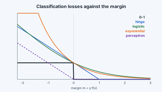
Why not minimise the 0-1 loss?

The 0-1 loss is a step: flat at 1 for every mistake, flat at 0 for every correct point. Its gradient is zero almost everywhere, so gradient methods get no signal, and minimising it over linear classifiers is NP-hard on non-separable data (Module 7). So every practical method replaces it with a surrogate loss: something convex, so that optimisation is reliable, and ideally an upper bound on the 0-1 loss, so that driving the surrogate down drives the training error down too. Hinge, logistic and exponential losses all satisfy both.

What the shapes reveal

Correct, comfortable points ( $m \ge 1$ ). Hinge loss is exactly zero: once a point is outside the margin, the SVM ignores it entirely. That is the source of its sparsity (only support vectors matter). Logistic and exponential losses never quite reach zero, so every point keeps a small influence, which is why logistic regression's solution depends on all the data.

Correct but close points ( $0 < m < 1$ ). Hinge, logistic and exponential losses all still charge something, pushing for a margin. The perceptron loss charges nothing: any correct point is fine, however close. That is why the perceptron settles for the first separating boundary it finds.

Confident mistakes ( $m \ll 0$ ). Hinge, logistic and perceptron losses grow linearly; the exponential loss grows exponentially. That is why AdaBoost is so sensitive to mislabelled points (one wildly wrong point can dominate the loss) while logistic regression and the SVM are more robust.

Points that are too correct ( $m > 1$ ). The squared loss $(1 - m)^2$ rises again: a point with $m = 3$ costs as much as one with $m = -1$ . Least squares on ±1 labels therefore pulls its boundary towards easy, far-away points, which is the failure seen in Module 7. It is the only loss in the table that is not decreasing in the margin, and it is a poor choice for classification.

The common recipe

Almost every method in this course is an instance of

\min_{f}\; \sum_{i=1}^{n} \ell\big(y_i f(x_i)\big) \;+\; \lambda\,\Omega(f),

a loss on each training point's margin plus a regulariser $\Omega$ that limits complexity.

Method	Loss $\ell$	Regulariser $\Omega$	Model $f$
Ridge regression	squared	$\lVert w\rVert^2$	linear
Logistic regression	logistic	$\lVert w\rVert^2$ (usually)	linear
Soft-margin SVM	hinge	$\lVert w\rVert^2$	linear or kernel
AdaBoost	exponential	number of rounds	sum of stumps
Gradient boosting	any	rounds, depth, learning rate	sum of trees

Choosing a method is largely choosing a loss (how to treat near and wrong points), a regulariser (what "simple" means) and a model family (what shapes are possible). The final chapters take the model family one step further: instead of fixing the features, learn them.

EasyLoss functions

Compute the hinge, logistic (base 2) and exponential losses at margins m = 2, 0.5 and −2.

MediumLoss functionsSVM

Why does the hinge loss lead to sparse solutions (support vectors) while the logistic loss does not?

MediumLoss functionsLeast squares