The Maximum-Margin Classifier

Of all the hyperplanes that separate the data, choose the one with the widest margin. Fixing the scale so the closest points satisfy y(w·x + b) = 1 makes the margin 2/‖w‖, so maximising it becomes the convex problem: minimise ½‖w‖² subject to yᵢ(w·xᵢ + b) ≥ 1. Only the points on the margin determine the answer.

On separable data the perceptron stops at the first boundary that works, and different runs stop at different boundaries. Some of them skim past training points; others sit comfortably in the middle of the gap. Intuitively the middle is safer: a new point that is slightly different from the training points is less likely to land on the wrong side. The perceptron's own mistake bound, $(R/\gamma)^2$ , said the same thing in mathematics: a wide margin makes a problem easy. The support vector machine (SVM) turns the intuition into an objective.

The margin of a hyperplane

Take a hyperplane $w^\top x + b = 0$ (now with an explicit intercept $b$ ). The distance from a point $x_i$ to it is

\frac{|w^\top x_i + b|}{\lVert w \rVert} .

If the hyperplane classifies $x_i$ correctly, $y_i(w^\top x_i + b) > 0$ , so the distance can be written without the absolute value as $\frac{y_i(w^\top x_i + b)}{\lVert w \rVert}$ . The margin of the hyperplane is its distance to the closest training point. We want the separating hyperplane whose margin is largest:

\max_{w,\, b}\; \min_{i}\; \frac{y_i(w^\top x_i + b)}{\lVert w \rVert} .

Two classes of points separated by a solid line, with two dashed parallel lines through the closest points of each class, forming an empty street of width 2 over the norm of w; the points on the dashed lines are circled as support vectors — The maximum-margin hyperplane sits in the middle of the widest empty street between the classes. The circled points on the street's edges are the support vectors.

Fixing the scale

The pair $(w, b)$ and any rescaled pair $(cw, cb)$ with $c > 0$ describe the same hyperplane, so we are free to choose a scale. Choose it so that the closest points satisfy

y_i(w^\top x_i + b) = 1 ,

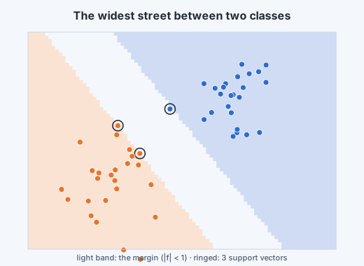
and every point satisfies $y_i(w^\top x_i + b) \ge 1$ . With this choice the closest points are at distance $1/\lVert w \rVert$ , and the empty "street" between the two classes, bounded by the parallel hyperplanes $w^\top x + b = \pm 1$ , has width

\text{margin width} = \frac{2}{\lVert w \rVert} .

Maximising $2/\lVert w\rVert$ is the same as minimising $\lVert w\rVert$ , or, more conveniently, $\tfrac12\lVert w \rVert^2$ . The problem becomes

\begin{aligned} \min_{w,\, b}\quad & \tfrac12\lVert w \rVert^2 \\ \text{subject to}\quad & y_i(w^\top x_i + b) \ge 1, \qquad i = 1, \dots, n. \end{aligned}

This is the hard-margin SVM. The objective is a convex quadratic (a bowl) and the constraints are linear, so it is a convex quadratic program: it has a single global optimum, which standard solvers find reliably. Unlike the perceptron, the answer does not depend on the order of the data or the starting point.

Support vectors

At the optimum, most constraints are slack: most points sit strictly outside the street, with $y_i(w^\top x_i + b) > 1$ . Only the points exactly on the street's edges have their constraints active. These are the support vectors. They alone determine the solution: delete any other point (or move it anywhere outside the street) and the optimal hyperplane does not change, while moving a support vector moves the hyperplane.

This is the SVM's version of compression. A data set of a million points may have only a few hundred support vectors, and the classifier is completely described by them. The next chapter makes this precise through the dual problem, which also opens the door to kernels.

Try it yourself

Machine Learning Lab: support vector machines →

Choose "Hard margin (large C)" on the "Apart" data. The light band is the street, the ringed points are support vectors, and the margin width is shown as 2/‖w‖.

Why a wide margin generalises

There are several ways to see why maximising the margin helps on new data.

Robustness. Each training point could be moved by up to the margin in any direction without being misclassified. If new points are noisy copies of training points, a wide margin absorbs the noise.
Few mistakes are possible. The perceptron bound $(R/\gamma)^2$ shows that a large margin relative to the data's size means a simple problem.
Capacity control. Learning theory shows that the set of classifiers with margin at least $\gamma$ on data of radius $R$ is effectively limited by $R^2/\gamma^2$ , regardless of the number of features. That is why SVMs can work in very high (even infinite) dimensional feature spaces without overfitting, provided the margin is wide.

The hard-margin SVM has one fatal flaw: if the data is not separable, the constraints cannot all be satisfied and the problem has no solution. A single mislabelled point can do that. The soft margin, two chapters on, fixes it.

MediumSVMMargin

Points (2, 2) with label +1 and (0, 0) with label −1. Find the maximum-margin hyperplane by inspection and verify the constraints.

EasySVMOptimisation

Why do we minimise ½‖w‖² instead of maximising 1/‖w‖ directly?

EasySVMSupport vectors