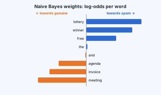
Naive Bayes

Naive Bayes estimates each class's prior and per-feature probabilities by counting, then classifies with Bayes' rule in log space. A word never seen in one class gets probability zero and vetoes that class, which Laplace smoothing fixes by adding pseudo-counts. For binary features its decision function is linear: a weighted vote of log-odds, one per feature.

The last chapter set up the generative story for classifying emails and showed that it is only practical with an assumption: given the class, the words appear independently. This chapter turns that assumption into a working classifier, fixes its one serious flaw, and shows that its decision rule is, surprisingly, a straight line.

Training by counting

The model has three kinds of parameters for a binary problem with binary features $x \in \{0, 1\}^d$ :

$\hat p = P(y = 1)$ , the prior probability of spam;
$\hat p^{\,1}_j = P(x_j = 1 \mid y = 1)$ , the probability that word $j$ appears in spam;
$\hat p^{\,0}_j = P(x_j = 1 \mid y = 0)$ , the probability that word $j$ appears in genuine mail.

Each is a coin-flip probability, and its maximum likelihood estimate is a frequency:

\hat p = \frac{\#\{\text{spam emails}\}}{n}, \qquad \hat p^{\,1}_j = \frac{\#\{\text{spam emails containing word } j\}}{\#\{\text{spam emails}\}},

and likewise for $\hat p^{\,0}_j$ using the genuine emails. Training is a single pass over the data, counting. That speed, and the ability to update the counts as new mail arrives, made naive Bayes the first widely deployed spam filter.

Predicting

For a new email $x$ , Bayes' rule with the independence assumption gives

P(y = 1 \mid x) \;\propto\; \hat p \prod_{j=1}^{d} \big(\hat p^{\,1}_j\big)^{x_j}\big(1 - \hat p^{\,1}_j\big)^{1 - x_j},

and similarly for $y = 0$ with $1 - \hat p$ and $\hat p^{\,0}_j$ . Predict the class with the larger value. In practice, multiply thousands of small probabilities and the result underflows to zero, so compare log scores instead:

\text{score}_y(x) = \ln P(y) + \sum_{j=1}^{d} \Big[x_j \ln \hat p^{\,y}_j + (1 - x_j)\ln\big(1 - \hat p^{\,y}_j\big)\Big].

A tiny example

Training data: 4 spam and 6 genuine emails. The word "lottery" appears in 3 of the 4 spam emails and 1 of the 6 genuine ones; "meeting" appears in 1 spam and 4 genuine. A new email contains "lottery" but not "meeting".

\begin{aligned} \text{spam:}\quad & 0.4 \times \tfrac{3}{4} \times \big(1 - \tfrac14\big) = 0.4 \times 0.75 \times 0.75 = 0.225 \\ \text{genuine:}\quad & 0.6 \times \tfrac{1}{6} \times \big(1 - \tfrac46\big) = 0.6 \times 0.167 \times 0.333 = 0.033 \end{aligned}

Normalising, $P(\text{spam} \mid x) = 0.225 / (0.225 + 0.033) \approx 0.87$ . Spam.

The zero-count problem

Suppose the word "invoice" appeared in some genuine emails but in none of the spam emails in the training set. Then $\hat p^{\,1}_{\text{invoice}} = 0$ , and any new email containing "invoice" gets spam probability exactly zero, no matter how many other spam words it contains: one factor of zero wipes out the whole product. A spammer only has to include one word that never happened to appear in the training spam. The same thing happens for a word that appears in every email of a class (then $1 - \hat p = 0$ for emails without it).

This is the overconfidence of maximum likelihood on small counts, met in Module 5 with three heads in three flips. The fix is the same one: a prior.

Laplace smoothing

Pretend that, before seeing any data, we saw every word appear once and not appear once in each class. The estimates become

\hat p^{\,y}_j = \frac{\#\{\text{class-}y\text{ emails containing word } j\} + 1}{\#\{\text{class-}y\text{ emails}\} + 2} .

This is Laplace smoothing (add-one smoothing), the posterior mean under a flat $\text{Beta}(1, 1)$ prior. No estimate can now be exactly 0 or 1, so no single word can veto a class. With plenty of data the added counts make almost no difference; with sparse counts they keep the model sensible. A more general version adds $\alpha$ instead of 1 to each count, with $\alpha$ chosen by validation.

The decision function is linear

Compare the two log scores: predict spam when $\text{score}_1(x) > \text{score}_0(x)$ . Collect the terms that multiply each $x_j$ :

\text{score}_1(x) - \text{score}_0(x) = \underbrace{\ln\frac{\hat p}{1 - \hat p} + \sum_j \ln\frac{1 - \hat p^{\,1}_j}{1 - \hat p^{\,0}_j}}_{b} \;+\; \sum_{j=1}^{d} \underbrace{\ln\frac{\hat p^{\,1}_j\,(1 - \hat p^{\,0}_j)}{\hat p^{\,0}_j\,(1 - \hat p^{\,1}_j)}}_{w_j}\; x_j .

So naive Bayes predicts spam exactly when

w^\top x + b > 0 :

a linear classifier. Each word casts a vote $w_j$ equal to its log-odds ratio: positive if the word is relatively more common in spam, negative if more common in genuine mail, near zero if it is equally common in both. The intercept $b$ carries the prior and the baseline. This makes naive Bayes easy to interpret: the largest positive weights are the "spammiest" words.

It also places naive Bayes in the same family as logistic regression and the perceptron, which also predict with $\operatorname{sign}(w^\top x + b)$ . They differ in how they choose $w$ : naive Bayes fits each class's data separately and derives the boundary; logistic regression chooses $w$ directly to fit the labels. When the independence assumption is badly wrong (for example, a duplicated feature gets counted twice), naive Bayes's weights are distorted while logistic regression adjusts for the redundancy.

A horizontal bar chart of words with their log-odds weights: lottery, winner and free have large positive bars towards spam; meeting, invoice and agenda have negative bars towards genuine mail; and, the and is have bars near zero — Naive Bayes as a linear classifier. Each word's weight is its log-odds ratio between the classes; the email's score is the sum of the weights of the words it contains, plus a baseline.

MediumNaive BayesLaplace smoothing

Using the example above but with Laplace smoothing, recompute P(spam | email with 'lottery' and not 'meeting').

EasyNaive Bayes

Why does one unseen word break an unsmoothed naive Bayes classifier?

MediumNaive BayesLinear classifiers