From Perceptrons to Neural Networks

A neural network stacks layers of linear maps and non-linear activations, so it learns its own features instead of relying on a fixed kernel. One hidden layer already solves XOR, and wide enough networks can approximate any continuous function. The parameters are learned by gradient descent on a loss, with backpropagation computing the gradients layer by layer via the chain rule.

Every classifier in this course has the same weakness at its core: it is linear in some fixed set of features. Kernels and feature maps make those features richer, but someone still has to choose them: a polynomial of degree 3, an RBF of width $\sigma$ , a set of tree splits. Neural networks take the last step: they learn the features from data, along with the classifier that uses them.

The single neuron, revisited

A logistic regression model is already a tiny network: a single neuron that computes a weighted sum of its inputs and passes it through a non-linear activation function,

a = \sigma(w^\top x + b).

The perceptron is the same neuron with a step function instead of the sigmoid. Both draw a single linear boundary, so neither can solve XOR (two classes in opposite quadrants), as Minsky and Papert pointed out.

Hidden layers

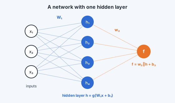
Put several neurons side by side, and feed their outputs into another neuron:

h = g\big(W_1 x + b_1\big), \qquad f(x) = w_2^\top h + b_2 .

The hidden layer $h$ is a vector of $k$ neurons, each computing its own weighted sum of the inputs followed by an activation $g$ (sigmoid, $\tanh$ , or most commonly today the ReLU, $g(z) = \max(0, z)$ ). The output is a linear function of the hidden values. In the language of this course: the hidden layer is a learned feature map $\phi(x) = g(W_1x + b_1)$ , and the output layer is a linear model on those features. Unlike a kernel, $\phi$ is not fixed in advance; its parameters $W_1, b_1$ are trained together with the output weights.

XOR with one hidden layer

Two hidden ReLU neurons are enough for XOR on inputs $x_1, x_2 \in \{0, 1\}$ :

h_1 = \max(0,\; x_1 + x_2), \qquad h_2 = \max(0,\; x_1 + x_2 - 1), \qquad f = h_1 - 2h_2 .

Check the four inputs: $(0,0)$ gives $0 - 0 = 0$ ; $(1,0)$ and $(0,1)$ give $1 - 0 = 1$ ; $(1,1)$ gives $2 - 2 = 0$ . The output is 1 exactly for the XOR-true inputs. The hidden layer has transformed the inputs into features in which the classes are linearly separable, which is what a kernel would do, but here the transformation is learned.

A network diagram with three input nodes, a hidden layer of four nodes, and one output node, with every input connected to every hidden node and every hidden node to the output; labels mark the weight matrices W1 and w2 and the activation g — A network with one hidden layer. Each hidden neuron computes g(weighted sum of inputs); the output is a weighted sum of the hidden values. The hidden layer is a feature map learned from data.

How powerful is one hidden layer?

The universal approximation theorem says that a network with a single hidden layer and enough neurons (with any reasonable non-linear activation) can approximate any continuous function on a bounded region as closely as you like. So one hidden layer is enough in principle. In practice, deep networks with many layers represent many functions with far fewer neurons, because each layer builds features out of the previous layer's features (edges, then textures, then parts, then objects, in an image network).

Learning the parameters

A network's parameters are all its weights and biases. Training chooses them to minimise a loss on the training data, exactly as before: squared error for regression, cross-entropy (the logistic loss, or its softmax version for many classes) for classification, usually plus an L2 penalty (called weight decay).

Two things change from the models earlier in the course.

The loss is not convex. Because the parameters sit inside non-linear functions of other parameters, the loss surface has many local minima and saddle points. There is no closed form and no guarantee of the global optimum. Remarkably, stochastic gradient descent on large networks usually finds solutions that generalise well anyway.
Gradients need an algorithm. A network may have millions of parameters. Backpropagation computes the gradient of the loss with respect to all of them efficiently by applying the chain rule layer by layer, from the output back to the input. One forward pass computes the predictions; one backward pass computes every partial derivative, at roughly the cost of a second forward pass.

For the one-hidden-layer network with squared loss $\tfrac12(f - y)^2$ , the chain rule gives, for example,

\frac{\partial\,\text{loss}}{\partial w_2} = (f - y)\,h, \qquad \frac{\partial\,\text{loss}}{\partial W_1} = \big[(f - y)\, w_2 \odot g'(W_1x + b_1)\big]\, x^\top ,

where $\odot$ is element-wise multiplication. The error signal $(f - y)$ flows backwards through $w_2$ and the activation's derivative to reach the first layer's weights.

Try it yourself

Deep Learning Lab: network lab →

Build a small network, train it on a dataset no line can separate, and watch the hidden layer bend the decision boundary.

Where neural networks fit

Neural networks are not a break from the ideas of this course; they combine them. A network is a learned feature map (Module 3's motivation) followed by a linear model (Modules 6 and 9), trained by gradient descent (Module 6) on a surrogate loss (this module), with weight decay as regularisation (ridge, from Module 6). What they add is the ability to learn representations from raw data such as pixels, audio and text, at a scale where hand-designed features fail.

The trade-offs are real. Networks need much more data and computation, have many hyperparameters, and are harder to interpret than a tree or a logistic regression. On small tabular data sets, gradient-boosted trees still often win. On images, speech and language, deep networks dominate. Our Deep Learning course builds them from the single neuron up, and the Large Language Models course follows them all the way to transformers.

MediumNeural networksXOR

Verify that the network h₁ = ReLU(x₁ + x₂), h₂ = ReLU(x₁ + x₂ − 1), f = h₁ − 2h₂ computes XOR, and explain why no single neuron can.

MediumNeural networksKernels

In what sense is a hidden layer a learned kernel?

MediumNeural networksOptimisation