PCA in Practice: Eigenfaces and Two Limits

PCA earns its place by working on real data. This chapter shows it doing something striking with photographs of faces, then looks honestly at two things it does badly. Fixing the first one, a matter of speed, will hand us the key to fixing the second, a matter of shape.

Eigenfaces

Take a large collection of grey-scale photographs of faces, all the same size and all looking straight at the camera. A photo is a grid of pixels, each a brightness value from 0 to 255. Read the grid row by row into one long list and each photo becomes a vector. A modest 180 × 180 image already gives a vector with more than 32,000 coordinates, so the data set is a cloud of points in a space with tens of thousands of dimensions.

Run PCA on it. Each principal component is itself a vector with the same number of coordinates as an image, so it can be folded back into a grid and viewed as a picture. These pictures are called eigenfaces.

• The first eigenface looks like a blurry, generic face: the direction along which face images vary most is, roughly, "how face-like and how brightly lit".
• Later eigenfaces add detail: the outline of the nose, the shape of the mouth, shadows around the eyes, the effect of light from one side.

Now take a new face, one that was not in the data set, and reconstruct it from only its first $k$ coefficients. With 25 components you get a face, but not recognisably this face. Somewhere around a few hundred components the person becomes recognisable, and adding more only sharpens fine detail. The image had tens of thousands of numbers, but a few hundred carry what identifies the person: roughly a hundredfold compression. This is why PCA is often used as a first step before a classifier: train the classifier on a few hundred coefficients instead of tens of thousands of pixels.

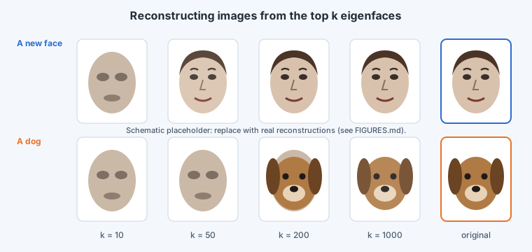
A revealing experiment: reconstruct a photo of a dog from the same face components. With a few hundred components the result looks like the most dog-like human face, because the top directions describe how faces vary, not how dogs vary. Only with many more components does the dog appear. A random noise image would need every single component. PCA learns the subspace where this kind of data lives; points from elsewhere fit it badly, and that misfit is itself useful (it is the basis of PCA-based anomaly detection).

Limit 1: too many features

The expensive step in PCA is the eigen-decomposition of the $d \times d$ covariance matrix, which for a general matrix costs on the order of $d^3$ operations. With $d$ in the tens of thousands, $d^3$ is in the trillions. In the face example, though, there are often fewer images than pixels: $n < d$. Can we pay for $n$ instead of $d$?

Every principal component is a combination of the data points

Stack the centred data points as the columns of a matrix:

Take an eigenvector $w$ of $C$ with a non-zero eigenvalue $\lambda$, so $Cw = \lambda w$. Writing out $C$ and dividing by $\lambda$:

So every principal component is a weighted sum of the data points, $w = X\alpha$ for some weight vector $\alpha \in \mathbb{R}^n$. That is natural: the directions of variation of a data set can only be built from the data. The formula for $\alpha$ is useless as it stands (it needs $w$, which we are looking for), but it tells us what to search for: $n$ weights instead of $d$ coordinates.

An n × n eigenproblem

Substitute $w = X\alpha$ into $\tfrac{1}{n}XX^\top w = \lambda w$:

Multiply both sides on the left by $X^\top$ and write $K = X^\top X$, an $n \times n$ matrix:

Any $\alpha$ satisfying the simpler equation

satisfies this one too. So $\alpha$ is an eigenvector of $K$. A linear algebra fact makes this consistent: $XX^\top$ ($d \times d$) and $X^\top X$ ($n \times n$) have the same non-zero eigenvalues (both come from the singular values of $X$). The eigenvalues of $K$ are therefore exactly $n\lambda_1, n\lambda_2, \dots$, the scaled eigenvalues of $C$.

Getting the length right

An eigenvector is only defined up to scale, but we need $\lVert w \rVert = 1$:

If $\beta$ is a unit eigenvector of $K$ with eigenvalue $n\lambda$, then $\beta^\top K \beta = n\lambda$, so the right scaling is

The faster algorithm

1. Compute $K = X^\top X$ (the $n \times n$ matrix of dot products between centred points).
2. Eigen-decompose $K$: unit eigenvectors $\beta_1, \beta_2, \dots$ with eigenvalues $n\lambda_1 \ge n\lambda_2 \ge \dots$
3. Set $\alpha_k = \beta_k / \sqrt{n\lambda_k}$.
4. The principal components are $w_k = X\alpha_k$, and the coefficient of point $x_j$ on component $k$ is $x_j^\top w_k = \sum_i \alpha_{k,i}\,(x_i^\top x_j)$.

The eigen-decomposition now costs about $n^3$ instead of $d^3$. With 2,000 images of 32,000 pixels that is a saving of a factor of roughly $16^3 \approx 4{,}000$. When $n > d$, the ordinary covariance route is the cheaper one: always decompose the smaller matrix.

The observation that changes everything

Look at what the faster algorithm actually needs. Entry $(i, j)$ of $K$ is

the dot product of two data points, a measure of how similar they are. Step 4 also uses only dot products. The whole of PCA can be computed from the pairwise dot products of the data, without ever looking at the coordinates themselves. Keep that in mind; it is the hinge of the next module.

Limit 2: PCA only sees straight structure

PCA finds the best linear subspace: lines, planes and their higher-dimensional versions through the mean. Many relationships between features are not linear. Suppose three measured features obey $f_3 = f_1^2 + f_2^2$. The data then lies on a curved surface, a bowl, inside three-dimensional space. It is genuinely two-dimensional (two numbers fix a point on the bowl), but no flat plane fits a bowl. PCA will report a large error for every plane and conclude that all three dimensions are needed. The structure is there; PCA simply cannot see its shape.

Two quite different complaints, then: one about computing time, one about the kind of structure PCA can find. The surprising answer, in the next module, is that the trick we just used for the first one (needing only dot products) also solves the second.