Principal Component Analysis

The previous chapter ended with a precise goal: on centred data, find the unit vector $w$ whose line loses the least when every point is replaced by its projection. This chapter solves it, then follows the "repeat on the residuals" procedure to its end. The result is principal component analysis (PCA), one of the most widely used algorithms in data science.

From least error to a matrix problem

For a unit vector $w$, the squared error of point $x_i$ is the squared length of its residual. Averaging over the data set,

Expand one term, using $w^\top w = 1$:

The first term does not depend on $w$, so minimising $f$ is the same as maximising the other term:

Now rewrite $(x_i^\top w)^2$ as $w^\top x_i\, x_i^\top w$. Since $w$ does not depend on $i$, it moves outside the sum:

The $d \times d$ matrix

is the covariance matrix of the centred data. Entry $(j, k)$ is the average of feature $j$ times feature $k$: the variances of the features on the diagonal and their covariances off it. So the best line is the solution of

A standard result of linear algebra (the Rayleigh quotient, a case of the Courant–Fischer min-max theorem) answers this immediately: the maximum is the largest eigenvalue $\lambda_1$ of $C$, reached when $w$ is the corresponding eigenvector. To see why, note that $C$ is symmetric, so it has an orthonormal basis of eigenvectors $v_1, \dots, v_d$ with eigenvalues $\lambda_1 \ge \dots \ge \lambda_d$. Write $w = \sum_j a_j v_j$ with $\sum_j a_j^2 = 1$; then $w^\top C w = \sum_j \lambda_j a_j^2$, a weighted average of the eigenvalues that is largest when all the weight sits on $\lambda_1$.

The same line maximises variance

The quantity we maximise has a plain meaning. Project every centred point onto $w$ and collect the numbers $x_1^\top w, \dots, x_n^\top w$. Their average is $\big(\tfrac{1}{n}\sum_i x_i\big)^\top w = 0$, because the data is centred. Their variance is therefore just the average square:

So on centred data,

minimising reconstruction error = maximising the variance of the projections.

The two always add up to the same total, the average squared length of the points, $\tfrac{1}{n}\sum_i \lVert x_i \rVert^2$, which is fixed by the data. Whatever variance the line keeps, it does not lose as error, and vice versa.

Why should we want the projections spread out? Because a compressed representation is only useful if it still tells points apart. Project onto a direction across a long thin cloud and every point lands near the origin: the coefficients crowd together and the points become indistinguishable. Project along the cloud and the coefficients stay spread out, preserving the differences between points. Variance is our measure of how much distinguishing information survives.

Repeating on the residuals

Take the residuals after the first line: $x_i' = x_i - (x_i^\top w_1)\,w_1$. Every residual is perpendicular to $w_1$ (we checked this in the last chapter), so all of them live in the subspace orthogonal to $w_1$. The best line for the residuals therefore also lies in that subspace: any component along $w_1$ would only add error. Hence $w_2 \perp w_1$.

The same argument repeats. After $k$ rounds we have unit vectors $w_1, \dots, w_k$ that are mutually perpendicular, an orthonormal set. Working through the residuals shows that after round $k$ each point has had all its components along $w_1, \dots, w_k$ removed:

In $d$ dimensions there is room for only $d$ perpendicular directions, so after $d$ rounds every residual is zero, and each point is rebuilt exactly as

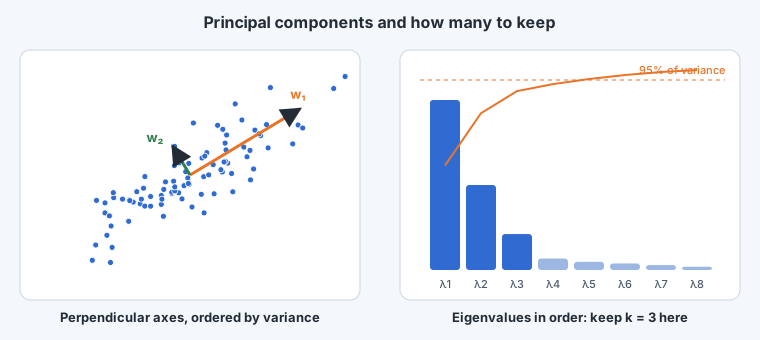
That is just a change of basis: from the standard axes to the new axes $w_1, \dots, w_d$. Linear algebra identifies these axes for us. The direction found in round $k$ is the eigenvector of $C$ with the $k$-th largest eigenvalue; the eigenvectors of a symmetric matrix are exactly an orthonormal basis. The $w_j$ are called the principal components.

Where the compression happens

A change of basis on its own saves nothing. The saving comes from stopping early. If the residuals become zero after $k$ rounds, the data lies exactly in a $k$-dimensional subspace, and each point needs only $k$ coefficients,

plus the $k$ shared directions. With $n = 100$ points in $d = 100$ dimensions that lie in a 3-dimensional subspace, we store $3 \times 100 + 3 \times 100 = 600$ numbers instead of $10{,}000$, and reconstruct everything exactly.

Real data never lies exactly in a subspace, so we also need to know when the remaining directions carry so little that we can drop them. The eigenvalues answer that. Since $C w_k = \lambda_k w_k$ and $w_k^\top w_k = 1$,

the variance captured along the $k$-th direction. Each eigenvalue is an average of squares, so it is never negative (the covariance matrix is positive semi-definite), and they decrease in order. A common rule of thumb keeps the smallest $k$ for which

that is, the top $k$ directions explain 95% of the variance. Plotting the eigenvalues in order (a scree plot) often shows an elbow: a few large values (signal) followed by a long tail of small ones (mostly noise).

The algorithm

1. Centre the data: subtract the mean $\mu$ from every point.
2. Form the covariance matrix $C = \tfrac{1}{n}\sum_i x_i x_i^\top$.
3. Compute its eigenvalues and eigenvectors, sorted from largest eigenvalue down.
4. Choose $k$, for example the smallest $k$ explaining 95% of the variance.
5. Represent each point by its $k$ coefficients $x_i^\top w_1, \dots, x_i^\top w_k$. To reconstruct, compute $\mu + \sum_{j \le k} (x_i^\top w_j)\, w_j$.

A worked picture: height and weight

Centre a set of heights and weights (in standard units) and suppose they rise together along the diagonal. The first principal component is then close to $w_1 = \tfrac{1}{\sqrt 2}[1, 1]^\top$, so each person's first coefficient is $\tfrac{\text{height} + \text{weight}}{\sqrt 2}$: a measure of overall size. The second is perpendicular, $w_2 = \tfrac{1}{\sqrt 2}[-1, 1]^\top$, giving $\tfrac{\text{weight} - \text{height}}{\sqrt 2}$: whether someone is heavy for their height.

In the original axes, knowing a person's height tells you a lot about their weight. In the new axes, knowing someone's overall size tells you nothing about whether they are heavy for their height. The projections onto principal components are uncorrelated: in the new basis the covariance matrix is diagonal, with the eigenvalues on the diagonal. PCA has found new features, combinations of the old ones, that each carry information the others do not.