Regression as Estimation, and Cross-Validation – Machine Learning Techniques

Assume labels are a linear function plus Gaussian noise: maximum likelihood then gives exactly least squares. Treating ŵ as an estimator, it is unbiased, and its mean squared error is σ² times the trace of (XXᵀ)⁻¹, which blows up when features are nearly dependent. Choosing between models needs an honest estimate of error on new data: cross-validation.

So far least squares has been justified by geometry: it is the closest point in the span of the features. Module 5 offers another justification. If we write down a probabilistic story for how the labels were generated, maximum likelihood should tell us how to fit it. For the most natural story, it gives least squares exactly, and the probabilistic view then lets us ask how good the fitted weights are.

A probabilistic model for the labels

Assume each label is a linear function of its features plus random noise:

y_i = w^\top x_i + \epsilon_i, \qquad \epsilon_i \sim \mathcal{N}(0, \sigma^2) \text{ independently}.

The features are taken as given; the randomness is all in the noise. Equivalently, given $x_i$ , the label is Gaussian with mean $w^\top x_i$ and variance $\sigma^2$ .

The log-likelihood of the observed labels is

\ell(w) = \sum_{i=1}^{n} \ln \mathcal{N}(y_i;\, w^\top x_i, \sigma^2) = -\frac{n}{2}\ln(2\pi\sigma^2) - \frac{1}{2\sigma^2}\sum_{i=1}^{n}\big(y_i - w^\top x_i\big)^2 .

The first term does not depend on $w$ . So maximising the likelihood over $w$ is the same as minimising the sum of squared errors:

\hat w_{\text{ML}} = \arg\min_w \sum_{i}(w^\top x_i - y_i)^2 = (XX^\top)^{-1}Xy .

Least squares is maximum likelihood under Gaussian noise. The squared error is not an arbitrary choice: it is what the Gaussian noise assumption implies. Change the assumption and the loss changes with it. Noise with heavier tails, the Laplace distribution, leads to minimising the sum of absolute errors instead, which is much less sensitive to outliers.

How good is ŵ?

The estimate $\hat w$ depends on the noise in the labels, so it is random: a fresh data set with new noise would give a different $\hat w$ . Treat it like any estimator and ask how close it lands to the true $w$ .

Substituting $y = X^\top w + \epsilon$ :

\hat w = (XX^\top)^{-1}X(X^\top w + \epsilon) = w + (XX^\top)^{-1}X\epsilon .

Unbiased: the noise has mean zero, so $\mathbb{E}[\hat w] = w$ . On average, least squares hits the truth.
Its spread: the covariance of $\hat w$ is $\sigma^2 (XX^\top)^{-1}$ , and the expected squared distance from the truth is

\mathbb{E}\big[\lVert \hat w - w \rVert^2\big] = \sigma^2\, \operatorname{tr}\big((XX^\top)^{-1}\big) = \sigma^2 \sum_{j=1}^{d} \frac{1}{\lambda_j},

where $\lambda_1, \dots, \lambda_d$ are the eigenvalues of $XX^\top$ .

That formula explains a familiar failure. If two features are nearly duplicates (say, height in centimetres and height in inches with a little rounding noise), $XX^\top$ has an eigenvalue close to zero, its reciprocal is huge, and the estimated weights swing wildly from one data set to the next, often as large positive and negative weights that nearly cancel. The predictions may still be fine on the training data, but the weights are meaningless and the predictions on new data are fragile. This is multicollinearity, and the next chapter's ridge regression is built to tame it.

Estimating error on new data

The quantity we care about is the expected squared error on new data, the generalisation error. Training error underestimates it, more and more as the model gets more flexible, so it cannot choose between a degree-3 and a degree-9 polynomial, or between penalty strengths. We need an estimate from data the model was not fitted to.

A validation set

The simplest approach: split the labelled data. Fit each candidate model on the training part, measure its error on the held-out validation part, and pick the best. Then (optionally) refit the chosen model on all the data. The drawback is waste: the validation points are not used for fitting, and with little data the estimate from a small validation set is itself noisy.

k-fold cross-validation

Cross-validation reuses every point for both purposes.

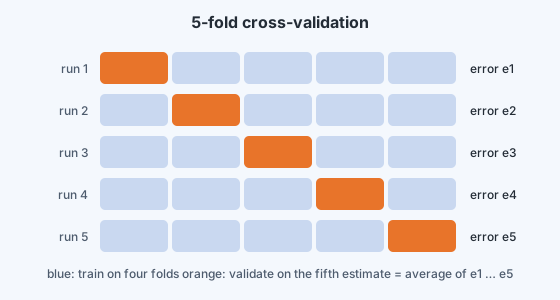
Split the data into $k$ equal folds (commonly $k = 5$ or $10$ ).
For each fold in turn, fit the model on the other $k - 1$ folds and measure its error on the held-out fold.
Average the $k$ errors. That average is the cross-validation estimate of generalisation error.

Run this for every candidate (each degree, each penalty strength) and choose the one with the lowest estimate. Every point is used for validation exactly once and for training $k - 1$ times.

With $k = n$ , each fold is a single point: leave-one-out cross-validation. It wastes almost nothing and, for least squares and ridge regression, can even be computed without refitting $n$ times (there is a closed-form shortcut using the diagonal of the "hat" matrix). Its estimate has low bias but can have high variance, which is one reason 5 or 10 folds are the common default.

Five rows, each showing the data split into five blocks; in each row a different block is shaded as the validation fold and the other four are training folds; the five validation errors are averaged — 5-fold cross-validation. Each fold takes one turn as validation data while the model is fitted on the other four; the five errors are averaged.

One rule matters more than any detail: the test data must not influence any choice. If the same data is used to choose the model and to report its accuracy, the reported accuracy is optimistic. Keep a final test set untouched until every decision has been made.

Try it yourself

Machine Learning Lab: regression →

The orange points are held-out data. Compare their error with the training error as you change the degree: the gap between the two curves is what validation measures.

MediumMLERegression

Labels have Laplace noise, p(ε) ∝ exp(−|ε|/b). What does maximum likelihood minimise?

MediumEstimatorsRegression

Why is ŵ unbiased under the Gaussian noise model, and what does unbiasedness not guarantee?

HardCross-validationModel selection

You use 10-fold cross-validation to pick a polynomial degree, then report the best cross-validation error as your model's expected accuracy. What is wrong?