Representation Learning: Compression as Understanding

If data points lie along a line, a representative vector and one coefficient per point describe them exactly. Real data never lies exactly on a line, so we replace each point by its projection (its closest proxy on the line) and look for the line that loses the least. Repeating on the leftovers gives a sequence of directions.

The first unsupervised problem we tackle is the vaguest-sounding one: given a set of data points, understand something useful about them. To make that precise we need three things: what a data point is, what "understand" means, and what "useful" means. The first is easy. The second is where the running theme of this course, comprehension is compression, does its work.

Data points are vectors

Throughout the course, a data set is a collection of $n$ points $x_1, x_2, \dots, x_n$ , each a vector of $d$ real numbers:

x_i \in \mathbb{R}^d .

Each coordinate is a feature. If we record the height, weight and age of 100 people, each person is a point in $\mathbb{R}^3$ and $n = 100$ . If we store 28-by-28 grey-scale images, each image is a point in $\mathbb{R}^{784}$ .

Understanding as compression

Here is a small data set of four points in two dimensions:

x_1 = \begin{bmatrix} -3 \\ 9 \end{bmatrix},\quad x_2 = \begin{bmatrix} 1 \\ -3 \end{bmatrix},\quad x_3 = \begin{bmatrix} 2 \\ -6 \end{bmatrix},\quad x_4 = \begin{bmatrix} 0 \\ 0 \end{bmatrix}.

How many numbers does a computer need to store it? The obvious answer is $4 \times 2 = 8$ . But look again: in every point, the second coordinate is exactly $-3$ times the first. If we spot that relationship, we can store the data differently:

one representative vector for the whole data set, say $w = [1, -3]^\top$ ;
one coefficient per point: $-3, 1, 2, 0$ .

Each point is the representative scaled by its coefficient: $x_3 = 2 \cdot w$ . That is $2 + 4 = 6$ numbers instead of 8, and nothing is lost: the data can be reconstructed exactly.

Six instead of eight is unimpressive, but the saving grows with the data. With a billion such points we would store $2 + 10^9$ numbers instead of $2 \times 10^9$ , almost exactly half. In $d$ dimensions, if every point is a multiple of one direction, the cost drops from $d \times n$ to $d + n$ . Finding that relationship is understanding something about the data, and the compression is the proof.

Two details will matter later.

The representative is not unique. Any non-zero vector along the same line works, with the coefficients rescaled to match. We are free to pick the one of length 1, which makes the formulas cleaner.
Lines through the origin. "Representative times coefficient" always describes a line through the origin (coefficient 0 gives the origin), so for now our lines pass through the origin.

When points leave the line

Real data is never this tidy. Add a fifth point, $x_5 = [1, -2]^\top$ , which is not on the line. Now no single representative reproduces all five points.

We could use two representatives, say $[1, 0]^\top$ and $[0, 1]^\top$ , and give every point two coefficients. That reconstructs everything exactly, but it costs $2n + 4$ numbers, which is more than storing the data directly. Exact reconstruction and compression are now in conflict, and one must give.

We give up exact reconstruction. Keep the line, and for the stray point find a proxy: a point on the line that stands in for it. We lose a little information (the gap between $x_5$ and its proxy), but we keep the compression. The natural choice of proxy is the point on the line closest to $x_5$ , because it loses the least. That point is the projection of $x_5$ onto the line.

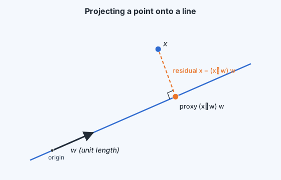
A line through the origin along a unit vector w, a point x off the line, its projection (x·w)w on the line, and the perpendicular residual from the projection to x — The proxy for x on the line through w is its projection (xᵀw)w. The residual x − (xᵀw)w is perpendicular to the line, which is why it is the shortest possible gap.

Finding the projection

Let the line be all multiples of a vector $w$ , and look for the multiple $c\,w$ closest to a point $x$ . The squared length of the gap is

f(c) = \lVert x - c\,w \rVert^2 = \lVert x \rVert^2 - 2c\,(x^\top w) + c^2 \lVert w \rVert^2 .

This is a parabola in $c$ . Setting its derivative to zero, $-2\,x^\top w + 2c\,\lVert w\rVert^2 = 0$ , gives

c^* = \frac{x^\top w}{\lVert w \rVert^2}, \qquad \text{proxy} = \frac{x^\top w}{\lVert w \rVert^2}\, w .

The numerator is the dot product of the point with the direction; the denominator is the squared length of the direction. If we choose $w$ with $\lVert w \rVert = 1$ , the denominator disappears:

\text{proxy} = (x^\top w)\, w, \qquad \text{coefficient} = x^\top w .

So with a unit representative, the coefficient of a point is simply its dot product with the representative. For our stray point, the unit vector along $[1, -3]^\top$ is $w = \tfrac{1}{\sqrt{10}}[1, -3]^\top$ , so the coefficient is $x_5^\top w = \tfrac{1 + 6}{\sqrt{10}} = \tfrac{7}{\sqrt{10}}$ and the proxy is $\tfrac{7}{10}[1, -3]^\top = [0.7, -2.1]^\top$ . The leftover, $x_5 - \text{proxy} = [0.3, 0.1]^\top$ , is perpendicular to $w$ , as it must be: $0.3 \cdot 1 + 0.1 \cdot (-3) = 0$ .

Which line?

So far someone handed us the line. In practice nobody tells us which points are "on the line" and which stray: every point strays a little. Height and weight are related, but no real class of 100 people lies exactly on a line.

Any line gives the same compression (one representative plus one coefficient per point), so compression cannot choose between lines. What differs is how much we lose. A line through the long axis of the cloud leaves short gaps; a line across it leaves long ones. That suggests the goal:

Find the unit vector $w$ whose line gives the smallest total reconstruction error over the data set.

The next chapter solves exactly this problem, and the solution turns out to be an eigenvector of a matrix built from the data.

Try it yourself

Machine Learning Lab: PCA →

Turn a line through a cloud of points, watch every point drop its projection onto it, and see the total error change with the angle.

The leftovers may still hold information

Suppose we find the best line. Are we done? Picture data in three dimensions that lies on a flat plane. The best single line lies somewhere in that plane, but every point's leftover (its residual, $x - (x^\top w)w$ ) also lies in the plane, and the residuals all point along one common direction. If the residuals were pure noise they would scatter in every direction; because they line up, they still contain structure.

That suggests a procedure:

Find the best line $w_1$ for the data.
Replace every point by its residual, $x_i - (x_i^\top w_1)\,w_1$ .
Find the best line $w_2$ for the residuals, and repeat.

Each round peels off one more direction. Before running it, one practical problem must be fixed: our lines pass through the origin, but a data cloud can sit far from the origin. A line through the origin may then fit badly even when the cloud is perfectly long and thin. The fix is to centre the data first, by subtracting the mean:

\mu = \frac{1}{n}\sum_{i=1}^{n} x_i, \qquad x_i \leftarrow x_i - \mu .

After centring, the origin sits in the middle of the cloud, and lines through the origin can follow its shape.

This procedure raises four questions, which the next two chapters answer:

How do we actually find the best line?
How many times should we repeat?
Where is the compression once there are several lines?
What representation of each point do we end up with?

EasyLinear algebraProjection

Show that, for a unit vector w, the residual x − (xᵀw)w is perpendicular to w.

MediumPCAPreprocessing

Why must the data be centred before searching for the best line through the origin?

MediumCompression