The last chapter found two problems with plain least squares. With flexible models it overfits, fitting noise with large weights. With nearly duplicate features its weights become wildly unstable. Both are cured by the same idea: penalise large weights. How you measure "large" (squared or absolute) gives two methods with strikingly different personalities.
Ridge regression
Add a penalty on the squared length of the weight vector:
with setting how much we care about small weights. The gradient is ; setting it to zero gives
Adding raises every eigenvalue of by , so the matrix is always invertible, and the tiny eigenvalues that made least squares unstable are lifted away from zero. (In practice the intercept is usually left unpenalised.)
Why it works
- It shrinks. In the eigenbasis of , ridge multiplies the least-squares component along the eigenvector with eigenvalue by . Directions the data pins down well (large ) are barely touched; poorly determined directions (small ), which are exactly where least squares went wild, are shrunk hard.
- Bias for variance. The ridge estimate is biased (pulled towards zero), but its variance is far smaller. Its expected squared error, bias² plus variance, can be much lower than that of the unbiased least-squares estimate. For a suitable it always is somewhat lower, in the sense that some beats whenever there is noise.
- It is MAP estimation. Put a Gaussian prior on the weights, , and keep the Gaussian noise model. The log-posterior is
so the MAP estimate is ridge regression with . Regularisation is a prior belief that the weights are small; the more noise relative to the prior spread, the stronger the penalty.
Lasso regression
Now penalise the sum of absolute values instead, the L1 norm:
This is lasso (least absolute shrinkage and selection operator). In Bayesian terms it is the MAP estimate under a Laplace prior, , which is sharply peaked at zero.
Lasso has no closed form, because has a corner at zero where it is not differentiable. It is still a convex problem, though, and is solved efficiently by coordinate descent (update one weight at a time, holding the rest fixed) or by subgradient and proximal methods. At the corner, the role of the derivative is played by a subgradient: any slope between and supports the function at zero.
The striking difference: exact zeros
With one weight and an orthonormal design, the two penalties act on the least-squares value like this:
Ridge scales every weight down but never to exactly zero. Lasso subtracts a fixed amount and clips at zero (soft-thresholding): any weight whose least-squares value is smaller than in size becomes exactly zero. With many features, lasso therefore returns a sparse model, using only a subset of the features. It performs feature selection and fitting in one step, which is invaluable when there are many candidate features and you suspect only a few matter.
The geometric picture
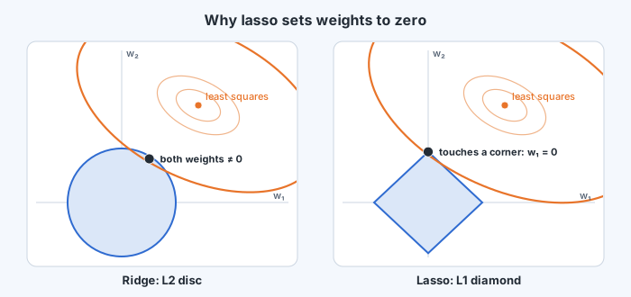
Write each problem as minimising squared error subject to a budget on the weights: for ridge, for lasso. The contours of the squared error are ellipses centred on the least-squares solution; the solution is where the smallest ellipse first touches the budget region. The ridge region is a disc, smooth everywhere, so the touching point is almost never on an axis. The lasso region is a diamond with corners on the axes, and an ellipse expanding towards it usually hits a corner first, where some weights are exactly zero. In high dimensions the L1 ball is all corners and edges, which is why sparsity is the rule rather than the exception.
Ridge or lasso?
| Ridge (L2) | Lasso (L1) | |
|---|---|---|
| Penalty | ||
| Prior | Gaussian | Laplace |
| Solution | closed form | iterative (coordinate descent) |
| Effect on weights | shrinks all, none exactly zero | sets many exactly to zero |
| Correlated features | spreads weight across them | tends to pick one and drop the rest |
| Best when | many small effects, collinearity | few features truly matter |
Elastic net combines both penalties, , to get sparsity while handling groups of correlated features gracefully. In every case, is chosen by cross-validation, and features should be standardised first, because both penalties treat all weights alike and a feature measured in large units would otherwise be penalised unfairly little.