The Dual Problem, Support Vectors and Kernels

The maximum-margin problem has a hidden second form, its dual, and the dual is where the SVM's best properties come from: it shows that the solution depends only on the support vectors, and that the data enters only through dot products, so kernels apply. Getting there takes one idea from optimisation, Lagrange multipliers for inequality constraints.

Constrained optimisation in brief

Take the general problem

Attach a multiplier $\alpha_i \ge 0$ to each constraint and form the Lagrangian

Here is the key observation. For a fixed $w$, maximise the Lagrangian over $\alpha \ge 0$. If $w$ breaks some constraint ($g_i(w) > 0$), raising $\alpha_i$ makes the Lagrangian infinite. If $w$ satisfies every constraint, every $g_i(w) \le 0$, so the best choice is to make each term zero, and the maximum is just $f(w)$. So

is exactly the original constrained problem: the inner maximum acts as an infinite penalty on infeasible $w$.

The dual problem swaps the order:

In general the dual's optimum is at most the original (primal) optimum. For convex problems such as the SVM, under a mild condition that holds whenever the data is separable, the two are equal (strong duality), so we may solve whichever form is more convenient.

The SVM dual

For the hard-margin SVM, $f(w) = \tfrac12\lVert w\rVert^2$ and the constraints are $1 - y_i(w^\top x_i + b) \le 0$. The Lagrangian is

Minimise over $w$ and $b$ by setting the derivatives to zero:

Substitute these back, and $w$ and $b$ disappear:

This is again a convex quadratic program, now in $n$ variables (one per training point) instead of $d + 1$.

What the dual reveals

1. The weights are a combination of training points

$w = \sum_i \alpha_i y_i x_i$. Once more, the solution lives in the span of the data, just as in kernel PCA and kernel regression.

2. Only support vectors count

At the optimum, the complementary slackness condition holds for every point:

Either $\alpha_i = 0$, or the constraint is tight, $y_i(w^\top x_i + b) = 1$, meaning the point lies exactly on the edge of the street. So $\alpha_i > 0$ only for support vectors; every other point has $\alpha_i = 0$ and drops out of $w = \sum_i \alpha_i y_i x_i$. This is the precise form of the statement in the last chapter: the classifier is built from the support vectors alone. The intercept follows from any support vector $s$: $b = y_s - w^\top x_s$.

3. The data appears only through dot products

Look at the dual objective: the training points enter only as $x_i^\top x_j$. And a prediction for a new point is

again only dot products, and only with the support vectors.

Kernel SVMs

So the kernel trick applies exactly as in Module 3. Replace every dot product by a kernel, $x_i^\top x_j \to k(x_i, x_j)$:

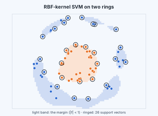
This finds the maximum-margin hyperplane in the kernel's feature space without ever computing the feature vectors. With a polynomial kernel the boundary in the original space is a polynomial curve; with the RBF kernel it can wrap around clusters of any shape, such as one ring inside another.

The kernel SVM also solves the cost problem of kernel regression. Kernel regression's prediction needed a kernel value with every training point; the SVM's needs only the support vectors, often a small fraction of the data.

Choosing the RBF width

The RBF kernel $k(x, x') = \exp(-\gamma\lVert x - x'\rVert^2)$ (here written with $\gamma = 1/2\sigma^2$) has a width parameter that matters a great deal. Small $\gamma$ (wide kernel): each support vector influences a large region, and the boundary is smooth, approaching a linear one. Large $\gamma$ (narrow kernel): influence is very local, the boundary can wrap around individual points, and the model overfits, with almost every point becoming a support vector. $\gamma$ and the soft-margin parameter $C$ (next chapter) are chosen together by cross-validation.