The EM Algorithm

Jensen's inequality turns the GMM's log-of-a-sum into a lower bound that is easy to maximise. Expectation-maximisation alternates two steps: the E step sets the bound to touch the log-likelihood by computing responsibilities, and the M step maximises the bound with weighted means, variances and proportions. The likelihood never decreases, and k-means is the hard-assignment limit.

The last chapter ended with a chicken-and-egg problem. If we knew which component produced each point, fitting the Gaussians would be easy; if we knew the Gaussians, working out which component produced each point would be easy. The expectation-maximisation (EM) algorithm alternates between the two and, unlike a hopeful guess, comes with a proof that every round improves the likelihood. The proof rests on one inequality about convex functions.

Convexity and Jensen's inequality

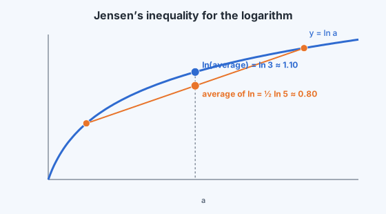
A function $g$ is convex if the chord between any two points on its graph lies on or above the graph: for $0 \le \lambda \le 1$ ,

g\big(\lambda a + (1 - \lambda) b\big) \le \lambda g(a) + (1 - \lambda) g(b) .

A bowl such as $x^2$ is convex. A function is concave if the inequality goes the other way (a dome); the logarithm is concave, because its second derivative $-1/x^2$ is negative.

Jensen's inequality extends the definition from two points to any weighted average. For a concave function such as $\ln$ , and weights $\lambda_k \ge 0$ that sum to 1,

\ln\Big(\sum_{k} \lambda_k\, a_k\Big) \;\ge\; \sum_{k} \lambda_k \ln a_k ,

with equality when all the $a_k$ are equal. In words: the log of an average is at least the average of the logs.

The concave curve y equals ln x, two points on it joined by a chord that lies below the curve; at the weighted average of the x values, the curve value ln of the average is above the chord value, the average of the logs — Jensen's inequality for the concave logarithm: the log of a weighted average (on the curve) is at least the weighted average of the logs (on the chord).

A lower bound on the log-likelihood

The GMM log-likelihood is a sum over points of the log of a sum over components. For each point $i$ , pick any weights $\lambda_{i1}, \dots, \lambda_{iK} \ge 0$ that sum to 1, and multiply and divide inside the sum:

\ln\Big(\sum_{k} \pi_k \mathcal{N}(x_i;\mu_k,\sigma_k^2)\Big) = \ln\Big(\sum_{k} \lambda_{ik}\,\frac{\pi_k \mathcal{N}(x_i;\mu_k,\sigma_k^2)}{\lambda_{ik}}\Big) \;\ge\; \sum_{k} \lambda_{ik}\,\ln\frac{\pi_k \mathcal{N}(x_i;\mu_k,\sigma_k^2)}{\lambda_{ik}} .

Summing over points gives a lower bound on the whole log-likelihood:

\ell(\theta) \;\ge\; B(\theta, \lambda) = \sum_{i=1}^{n}\sum_{k=1}^{K} \lambda_{ik}\Big[\ln \pi_k + \ln \mathcal{N}(x_i;\mu_k,\sigma_k^2) - \ln\lambda_{ik}\Big].

Two facts make this bound useful.

The bound is easy to maximise over $\theta$ . The log now acts directly on each Gaussian, so the awkward log-of-a-sum is gone. Each component's parameters appear in their own separate terms.
The bound can be made tight. Jensen's inequality is an equality when the terms inside are equal across $k$ , which happens when $\lambda_{ik}$ is proportional to $\pi_k\mathcal{N}(x_i;\mu_k,\sigma_k^2)$ . That is exactly the responsibility from the last chapter:

\lambda_{ik} = \frac{\pi_k \mathcal{N}(x_i;\mu_k,\sigma_k^2)}{\sum_{j}\pi_j\mathcal{N}(x_i;\mu_j,\sigma_j^2)} = P(z_i = k \mid x_i) .

The two steps

EM starts from a guess $\theta^{(0)}$ and repeats:

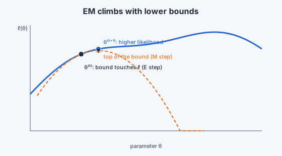
E step (expectation). With the current parameters, compute every responsibility $\lambda_{ik}$ . This makes the lower bound touch the log-likelihood at the current $\theta$ .

M step (maximisation). With the responsibilities fixed, maximise the bound over $\theta$ . Setting its derivatives to zero gives closed forms, each a weighted version of the single-Gaussian maximum likelihood answer. Writing $N_k = \sum_i \lambda_{ik}$ for the effective number of points in component $k$ :

\pi_k = \frac{N_k}{n}, \qquad \mu_k = \frac{1}{N_k}\sum_{i} \lambda_{ik}\, x_i, \qquad \sigma_k^2 = \frac{1}{N_k}\sum_{i} \lambda_{ik}\,(x_i - \mu_k)^2 .

Each point contributes to every component, in proportion to how responsible that component is for it. (In $d$ dimensions, the variance becomes the weighted covariance matrix $\Sigma_k = \tfrac{1}{N_k}\sum_i \lambda_{ik}(x_i - \mu_k)(x_i - \mu_k)^\top$ .)

Why the likelihood never goes down

Let $\theta^{(t)}$ be the current parameters and $\lambda^{(t)}$ the responsibilities computed from them. Then

\ell(\theta^{(t+1)}) \;\ge\; B(\theta^{(t+1)}, \lambda^{(t)}) \;\ge\; B(\theta^{(t)}, \lambda^{(t)}) \;=\; \ell(\theta^{(t)}) .

The first inequality is Jensen (the bound is always below the log-likelihood). The second holds because the M step chose $\theta^{(t+1)}$ to maximise the bound. The equality holds because the E step made the bound tight at $\theta^{(t)}$ . So each round can only raise the log-likelihood, or leave it unchanged. Like k-means, EM climbs steadily, and like k-means it can stop at a local maximum, so the starting point matters (a common choice is to initialise from a k-means solution).

The log-likelihood curve over a parameter, and a lower-bound curve that touches it at the current parameter; the maximum of the bound gives the next parameter, where a new bound touches again, climbing towards a peak — EM as climbing with lower bounds. The E step builds a bound that touches the log-likelihood at the current parameters; the M step jumps to the top of the bound. Repeating never lowers the likelihood.

Try it yourself

Machine Learning Lab: Gaussian mixtures and EM →

Press "One EM step" repeatedly. Watch the ellipses reshape, the colours blend where components overlap, and the log-likelihood curve rise and flatten, never falling.

EM and k-means

Put the two algorithms side by side.

	k-means	EM for a GMM
Assignment	hard: each point to its nearest mean	soft: responsibilities $\lambda_{ik}$
Update	plain mean of assigned points	weighted means, variances and proportions
Cluster shape	Voronoi cells, implicitly equal spread	each component has its own spread and weight
Objective	within-cluster squared distance falls	log-likelihood rises

k-means is in fact a limiting case of EM. Give every component the same small variance $\sigma^2$ and equal proportions, and let $\sigma^2 \to 0$ . The responsibilities then become 1 for the nearest mean and 0 for all others, the weighted means become plain means, and EM turns into Lloyd's algorithm. The probabilistic model adds what k-means lacked: clusters of different sizes and shapes, and an honest statement of uncertainty for points that sit between clusters.

HardEMGMM

Carry out one EM step by hand: points 1, 2, 9, 10 on a line, two components with means 2 and 8, variances 1, and equal proportions.

MediumEMConvergence

Why does EM never decrease the log-likelihood?

EasyJensenConvexity