The Perceptron

The perceptron learns a linear classifier sign(w·x) by cycling through the data and adding y·x to w whenever it makes a mistake. If the data is linearly separable with margin γ and radius R, it makes at most (R/γ)² mistakes before separating it perfectly; if not, it never settles.

Naive Bayes reached a linear classifier indirectly, by modelling each class and comparing them. The perceptron, proposed by Frank Rosenblatt in 1958, goes straight for the boundary. Its learning rule fits in one line, and it comes with one of the first and most elegant guarantees in machine learning.

A linear classifier

The perceptron predicts with a hyperplane through the origin:

h_w(x) = \operatorname{sign}(w^\top x) \in \{-1, +1\}.

(An intercept is handled, as before, by appending a constant feature 1.) The vector $w$ is perpendicular to the boundary $w^\top x = 0$ and points towards the positive side.

A point is classified correctly exactly when $y\,w^\top x > 0$ : the label and the score have the same sign. That product, $y\,w^\top x$ , will matter throughout the rest of the course; it is called the margin of the point (positive means correct, and larger means more comfortably correct).

The learning rule

Start with $w = 0$ . Repeatedly go through the training points; whenever a point is misclassified ( $y_i\,w^\top x_i \le 0$ ), update

w \;\leftarrow\; w + y_i\, x_i .

Stop when a full pass makes no mistakes.

Why does this help? After the update, the same point's margin becomes

y_i\,(w + y_i x_i)^\top x_i = y_i\,w^\top x_i + \lVert x_i \rVert^2 ,

larger by $\lVert x_i \rVert^2$ . The update rotates $w$ towards a misclassified positive point (or away from a misclassified negative one). It may break other points that were correct, so it is not obvious that the process ever ends. It does, if the data allows it.

Try it yourself

Deep Learning Lab: perceptron learning algorithm →

Watch the perceptron's boundary jump after each mistake and settle once every point is on the right side.

Linearly separable data

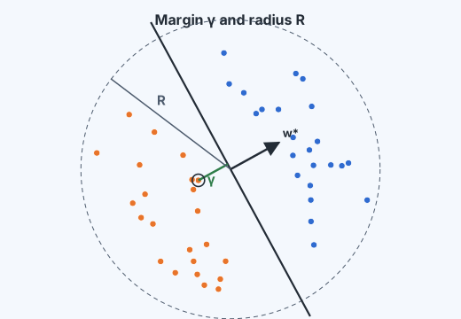
The data is linearly separable if some $w^*$ classifies every training point correctly. Then we can scale $w^*$ to unit length and ask how comfortably it separates the data. Define the margin of the data with respect to $w^*$ ,

\gamma = \min_{i}\; y_i\, w^{*\top} x_i > 0, \qquad \lVert w^* \rVert = 1 ,

the distance from the boundary to the closest point, and the radius of the data,

R = \max_i \lVert x_i \rVert .

The convergence theorem

If the data is linearly separable with margin $\gamma$ and radius $R$ , the perceptron makes at most $(R/\gamma)^2$ mistakes, and then classifies all the training points correctly.

The proof tracks two quantities after $k$ mistakes, $w_k$ being the weight vector at that point.

1. $w_k$ gains alignment with $w^*$ steadily. Each mistake on point $i$ adds $y_i x_i$ , so

w_{k}^\top w^* = w_{k-1}^\top w^* + y_i\, x_i^\top w^* \;\ge\; w_{k-1}^\top w^* + \gamma ,

since every point has margin at least $\gamma$ . Starting from $w_0 = 0$ , after $k$ mistakes $w_k^\top w^* \ge k\gamma$ .

2. $w_k$ grows slowly in length.

\lVert w_k \rVert^2 = \lVert w_{k-1} \rVert^2 + 2y_i\,w_{k-1}^\top x_i + \lVert x_i\rVert^2 \;\le\; \lVert w_{k-1}\rVert^2 + R^2 ,

because the middle term is $\le 0$ (it was a mistake) and $\lVert x_i\rVert^2 \le R^2$ . So $\lVert w_k\rVert^2 \le kR^2$ .

Combine them. Since $w^*$ has unit length, the Cauchy–Schwarz inequality gives $w_k^\top w^* \le \lVert w_k\rVert$ . So

k\gamma \;\le\; w_k^\top w^* \;\le\; \lVert w_k \rVert \;\le\; \sqrt{k}\,R \quad\Longrightarrow\quad k \;\le\; \frac{R^2}{\gamma^2} .

The alignment grows in proportion to $k$ , but the length only like $\sqrt{k}$ ; they cannot keep that up forever, so the mistakes must stop. The bound depends on neither the number of points nor the dimension, only on how wide the gap between the classes is relative to the size of the data. A wide margin means few mistakes. That idea, that the margin governs how hard a problem is, leads directly to support vector machines in Module 10.

The quantities in the perceptron bound. γ is the distance from a separating line to the nearest point; R is the radius of the data. At most (R/γ)² mistakes are possible.

Limits of the perceptron

Non-separable data. If no hyperplane separates the classes, some point is always misclassified, the updates never stop, and the final $w$ depends on where you happen to stop. Variants fix this: the pocket algorithm keeps the best $w$ seen so far, and the averaged perceptron predicts with the average of all the $w$ 's, which is far more stable.
Any separator will do. On separable data the perceptron stops at the first boundary that works, which may pass very close to some points. It has no preference for a boundary in the middle of the gap, so its predictions on new points near the classes can be fragile.
Only linear boundaries. Rosenblatt's critics, Minsky and Papert, emphasised in 1969 that a single perceptron cannot represent XOR. Kernels (the perceptron's updates only involve dot products, so it can be kernelised) and multi-layer networks (Module 11) both remove that limit.

The perceptron can also be seen as stochastic gradient descent on a particular loss, the perceptron loss $\max(0, -y\,w^\top x)$ , which is zero for every correctly classified point however close to the boundary. Module 11 compares it with the losses of the other classifiers.

MediumPerceptron

Run the perceptron (no intercept) on the points (1, 2) with label +1 and (2, −1) with label −1, starting at w = (0, 0).

EasyPerceptronConvergence

The data has radius R = 10 and is separable with margin γ = 0.5. What does the perceptron guarantee? What if every point is scaled by 3?

EasyPerceptron